Use `datashader` for time-series distribution plots

The following seems to demonstrate how we can use datashader to produce distribution plots rather quickly for large series:

import pickle

import datashader as ds
import datashader.transfer_functions as tf

import matplotlib.pyplot as plt

# Load posterior predictive estimates for a simulated series
with open("sample_pp_trace.pkl", "rb") as f:
    pp_trace = pickle.load(f)

pp_trace.observed_data
# <xarray.Dataset>
# Dimensions:  (dt: 8784)
# Coordinates:
#   * dt       (dt) datetime64[ns] 2020-02-11T01:00:00 ... 2021-02-11
# Data variables:
#     Y_t      (dt) int64 1955927 1870384 1793920 ... 1940015 1790022 1737292
# Attributes:
#     created_at:                 2021-09-21T20:21:14.864357
#     arviz_version:              0.11.2
#     inference_library:          pymc3
#     inference_library_version:  3.11.2

pp_trace.posterior_predictive
# <xarray.Dataset>
# Dimensions:     (beta_dim_0: 2016, chain: 1, draw: 100, dt: 8784, xi_0_dim_0: 2016, xi_1_dim_0: 2016)
# Coordinates:
#   * chain       (chain) int64 0
#   * draw        (draw) int64 0 1 2 3 4 5 6 7 8 9 ... 91 92 93 94 95 96 97 98 99
#   * dt          (dt) datetime64[ns] 2020-02-11T01:00:00 ... 2021-02-11
#   * beta_dim_0  (beta_dim_0) int64 0 1 2 3 4 5 ... 2010 2011 2012 2013 2014 2015
#   * xi_0_dim_0  (xi_0_dim_0) int64 0 1 2 3 4 5 ... 2010 2011 2012 2013 2014 2015
#   * xi_1_dim_0  (xi_1_dim_0) int64 0 1 2 3 4 5 ... 2010 2011 2012 2013 2014 2015
# Data variables:
#     S_t         (chain, draw, dt) int64 1 1 1 1 1 1 1 1 1 ... 1 1 1 1 1 1 1 1 1
#     beta        (chain, draw, beta_dim_0) float64 -0.3512 0.75 ... -0.2256
#     xi_0        (chain, draw, xi_0_dim_0) float64 0.0004301 ... -0.0001103
#     xi_1        (chain, draw, xi_1_dim_0) float64 -40.1 -4.832 ... 3.142 3.291
#     mu          (chain, draw, dt) float64 1.888e+06 1.862e+06 ... 1.477e+06
#     Y_t         (chain, draw, dt) float64 1.979e+06 1.799e+06 ... 1.491e+06
# Attributes:
#     created_at:                 2021-09-21T20:21:14.861233
#     arviz_version:              0.11.2
#     inference_library:          pymc3
#     inference_library_version:  3.11.2

df = pp_trace.posterior_predictive.Y_t[0].drop("chain").to_dataframe()
df = df.reset_index()
df.dt = df.dt.astype(int)

N_obs = pp_trace.posterior_predictive.dt.data.shape[0]

canvas = ds.Canvas(
    plot_width=N_obs,
    plot_height=300,
    # x_range=(ds_df.dt.min(), ds_df.dt.max()),
    y_range=(0.0, df["Y_t"].max()),
    x_axis_type="linear",
    y_axis_type="linear",
)

agg = canvas.points(df, "dt", "Y_t")
agg.coords.update({"dt": pp_trace.posterior_predictive.dt.data})

shade_res = tf.shade(agg, cmap="black", how="eq_hist")

res_img = tf.Image(shade_res)

plt.close()

fig, ax = plt.subplots(figsize=(10, 5))

qmesh = res_img.plot(cmap="Blues", ax=ax, label="posterior predictives")

ax.step(
    pp_trace.observed_data.dt.data,
    pp_trace.observed_data.Y_t.data,
    color="black",
    label="obs",
    alpha=0.7,
    linewidth=1.3,
)

# XXX: Don't use `ax.legend`; it might freeze the plot!
fig.legend()

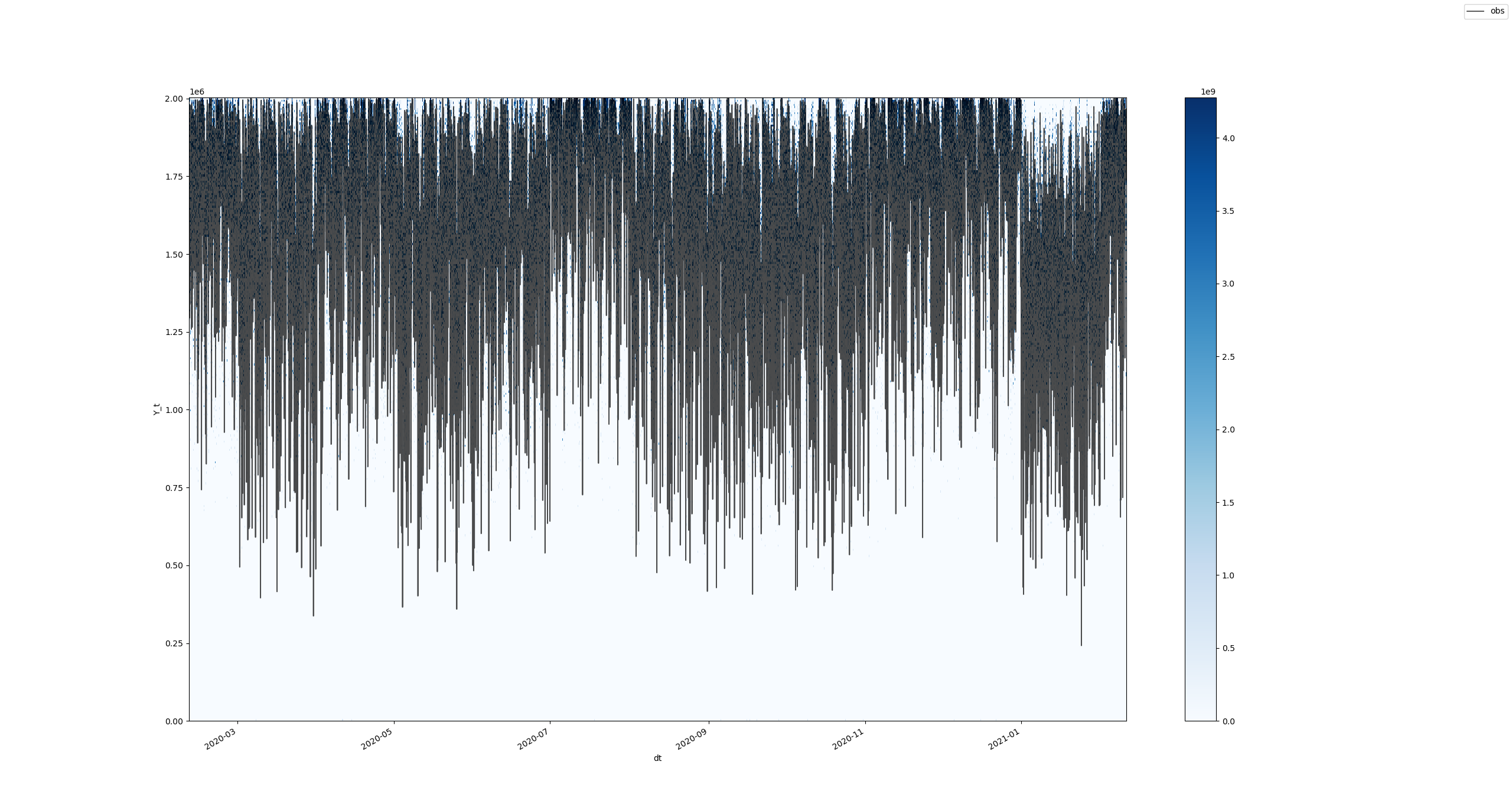
The whole picture won't look good for some obvious reasons, but, after zooming in, the results look similar to the ones we're producing (albeit with much more effort and less scalability): example-series-no-zoom

After zooming: example-series-zoomed

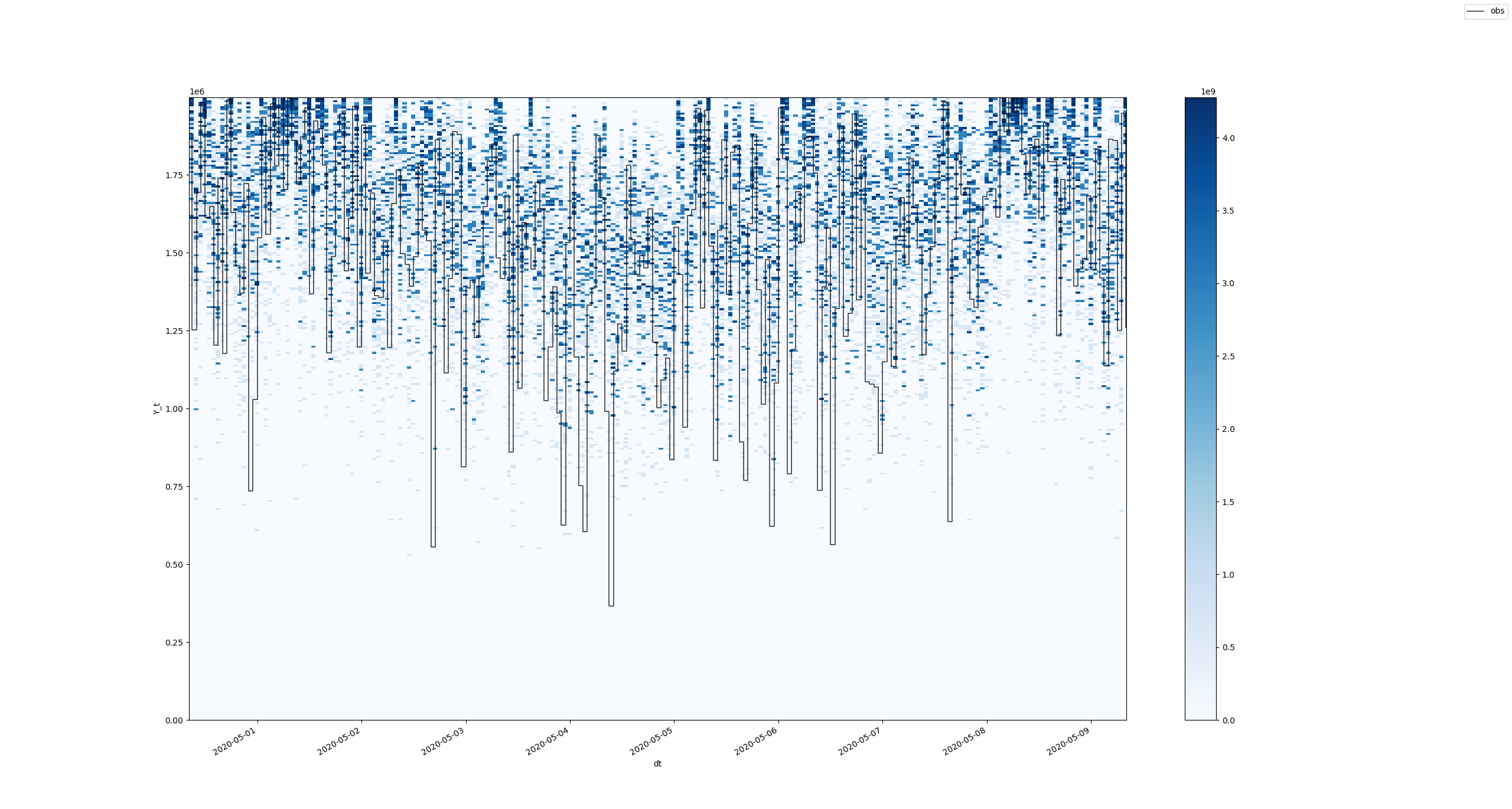
Let's try to improve these results and replace our current time-series histogram approach with this one.

AmpersandTV / pymc3-hmm

Use `datashader` for time-series distribution plots #93