Load SP trajectories in python

[loganbeal]

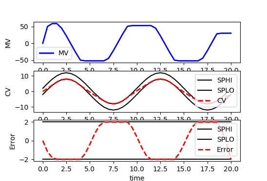
CV setpoint trajectories (tr or tr_hi/tr_lo) are reported in results.json and used in GUIs, but not loaded to python. It would be nice to read these into the associated python CV variables for local plotting.

When are these parameters reported?

• Only for CVs (does CV.STATUS matter) ?
• tr for cv_type=2 and tr_hi/tr_lo for cv_type=1 ?

While we're at it, there are a few other parameters in results.json that might be worth reading, such as bcv, tau, trs_hi, trs_lo, sp_hi, sp_lo, err_hi, err_lo, bias, wsp_hi, wsp_lo and cost. Some of these are not documented (eg what is the difference between tr_hi and trs_hi?). Some of them appear to be the same as constant values already reported (such as sp_hi and bias) -- are they different?

[APMonitor]

Those all look like great parameters to read in. There is a difference between tr_hi and trs_hi with trs_hi using a slack variable to calculate the trajectory. Some of the parameters change based on options selected such as when m.options.CV_TYPE=1 or m.options.CV_TYPE=2. Because these aren't used by many and they change based on the options, I've always thought of these as extra variables that someone can read in if interested.

m.solve()

# get additional solution information
import json
with open(m._path+'//results.json') as f:
    results = json.load(f)

plt.plot(m.time,results['v1.tr'],'k-',label='Reference Trajectory')

[APMonitor]

The tr_hi and tr_lo are for IMODE=6 when CV_TYPE=1 and tr is produced when CV_TYPE=2 for a squared error objective. I suggest that we keep those as a json import because of the complications of how different parameters are returned when modes switch. Here is an example of importing the results.json file with a custom reference trajectory.

import numpy as np
from random import random
from gekko import GEKKO
import matplotlib.pyplot as plt

# initialize GEKKO model
m = GEKKO()

# time
m.time = np.linspace(0,20,41)

# constants
mass = 500

# Parameters
b = m.Param(value=50)
K = m.Param(value=0.8)
# Manipulated variable
p = m.MV(value=0, lb=-100, ub=100)

# Reference trajectory
sine = 10*np.sin(m.time/20*4*np.pi)
traj = m.Param(value=sine)

# Controlled Variable
v = m.SV(value=0,name='v')

# Error
e = m.CV(value=0,name='e')

# Equations
m.Equation(mass*v.dt() == -v*b + K*b*p)
m.Equation(e==v-traj)

m.options.IMODE = 6 # control

# MV tuning
p.STATUS = 1 #allow optimizer to change
p.DCOST = 0.1 #smooth out MV
p.DMAX = 50 #slow down change of MV

# CV tuning
e.STATUS = 1 #add the CV to the objective
m.options.CV_TYPE = 1 #Dead-band
db = 2
e.SPHI = db #set point
e.SPLO = -db #set point
e.TR_INIT = 0 #setpoint trajectory
e.TAU = 5 #time constant of setpoint trajectory

# Solve
m.solve()

# get additional solution information
import json
with open(m.path+'//results.json') as f:
    results = json.load(f)

# Plot solution
plt.figure(figsize=(6,4))
plt.subplot(3,1,1)
plt.plot(m.time,p.value,'b-',lw=2,label='MV')
plt.legend(loc='best')
plt.ylabel('MV')
plt.subplot(3,1,2)
plt.plot(m.time,sine+db,'k-',label='SPHI')
plt.plot(m.time,sine-db,'k-',label='SPLO')
plt.plot(m.time,v.value,'r--',lw=2,label='CV')
plt.legend(loc='best')
plt.ylabel('CV')
plt.subplot(3,1,3)
plt.plot(m.time,results['e.tr_hi'],'k-',label='SPHI')
plt.plot(m.time,results['e.tr_lo'],'k-',label='SPLO')
plt.plot(m.time,e.value,'r--',lw=2,label='Error')
plt.legend(loc='best')
plt.ylabel('Error')
plt.xlabel('time')
plt.tight_layout()
plt.savefig('mpc.png',dpi=300)
plt.show()