weekly useful materials - 06/01 -

[GENZITSU]

AIOps研究録―SREのための
システム障害の自動原因診断 / SRE NEXT 2022

AIを用いてシステム運用効率化AIOpsにおいて障害の原因診断を行う手法を検討した発表。

オフラインで異常と判定されたメトリクスをグルーピングし、因果グラフを生成することで、原因診断を行う。

以下概要のスライドをペタペタ

本手法ではメトリクスの数や変数に対する個別のチューニングが不要となっている

手法の流れ

異常検知

クラスタリング

因果推論

コメント

一連の手法の流れ、及び各stepで考慮すべき事項が丁寧にまとめられていてとても勉強になる。

出典

AIOps研究録―SREのための
システム障害の自動原因診断 / SRE NEXT 2022

[GENZITSU]

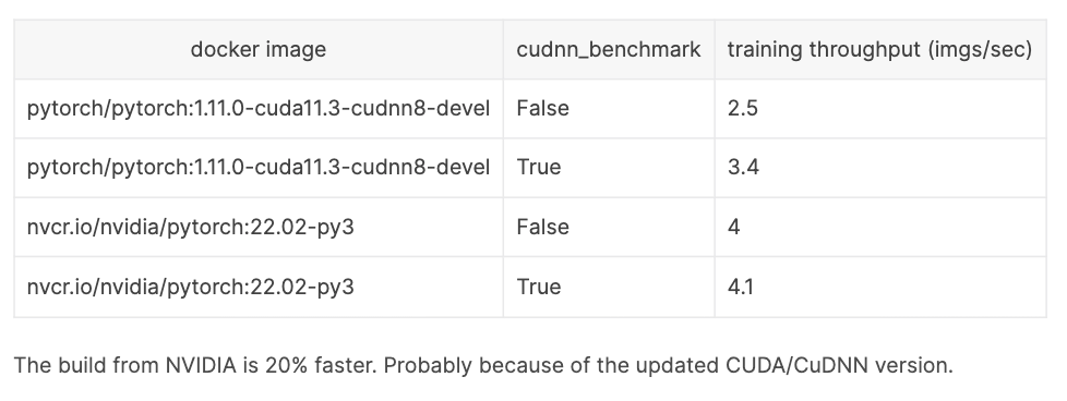
Lessons From Deploying Deep Learning To Production

自動運転ベンチャーのCruiseにて筆者が学んだ機械学習モデルのプロダクション運用で重要なことがストーリー形式で綴られている。

以下ためになった点の抜粋

プロダクション環境におけるMLは継続的な改善パイプラインが全てである

I used to think that machine learning was about the models. Actually, machine learning in production is about pipelines. One of the best predictors of success is the ability to effectively iterate on your model pipeline

in research and prototyping stages, the focus is on building and shipping a model. But as a system moves into production, the name of the game is in building a system that is able to regularly ship improved models with minimal effort. The better you get at this, the more models you can build!

継続的な改善パイプラインを達成するためには以下の要素を達成する必要がある

• Uncover problems in the data or model performance
• Diagnose why the problems are happening
• Change the data or the model code to solve these problems
• Validate that the model is getting better after retraining
• Deploy the new model and repeat

プロダクション環境からのフィードバックループを構築する

Set Up A Feedback Loop

フィードバックループには色々な種類があり

ドメインによっては正解データが継続的に手に入ることがある

Leverage domain-specific feedback loops. When available, these can be very powerful and efficient ways of getting model feedback. For example, forecasting tasks can get labeled data “for free” by training on historical data of what actually happened, allowing them to continually feed in large amounts of new data and fairly automatically adapt to new situations.

顧客からのエラー報告も役に立つ

Set up a workflow where a human can review the outputs of your model and flag when an error occurs. The most common way this occurs is when customers notice mistakes in the model outputs and complain to the ML team

モデルの革新度が低かったケースを取ってくるのも良い

The most general (but difficult) solution is to analyze model uncertainty about the data it is running on. A naive example is to look at examples where the model produced low confidence outputs in production. This can surface places where the model is truly uncertain, but it’s not 100% precise.

コメント

商用稼働が当たり前になった先の世界として非常に勉強になる。

出典

Lessons From Deploying Deep Learning To Production

[GENZITSU]

adversarial training.pptx

過学習の抑制手法として活用されているadversarial trainingの近年の手法がまとめられている。

いわゆる元祖

教師データ必要なやつ

Gradientをつかうやつ

最近のNLPコンペの上位解法で用いられたやつ

コメント

syntheticデータを用いると、それに過学習しやすくなってしまうので、ここら辺の手法で緩和できたりすると嬉しい

出典

adversarial training.pptx

[GENZITSU]

Happywhale 1st place solution

コンペの概要

こちらのEDAが参考になる

以下のような画像から鯨と海豚の個体識別を行うコンペティション

画像の枚数は5.1万枚で個体番号の他に種別の情報が付与されている

以下の分布のように個体や種別には大きな偏りがあり、中には1枚しか画像がない種別もあった

画像の中から鯨たちのbboxを導出し、そのbboxを用いてidentificationを訓練するというの基本的な流れ。

どうやらコンペティションの途中で、画像のどこに鯨やイルカがいて、体全体/尾びれなどのannotationを公開した参加者がいたようだ。

以下特徴的なところ

1. sub-center ArcFace with Dynamic margins のDyanmic marginをoptunaで最適化

sub-center ArcFace with Dynamic margins はGoogle Landmarkコンペの上位解法として用いられいたもので、Sub-center ArcFace: Boosting Face Recognition by Large-scale Noisy Web Faceという論文で提案されたもの。

概要は以下

ArcFaceとちがって重みにk個分の深みがでている。

このk個分の深みはデータセットの規模が大規模になることで出現するノイズに対応するために導入されたもの inter class の違いと intra classの違いの両方を考慮できる点でノイズに強くなるっぽい

However, this is not true especially when the dataset is in large scale. How to enable ArcFace to be robust to noise is one of the main challenges

そして難しいサンプルやnoisyなサンプルを自動的に分離することができるらしい

the proposed sub-center ArcFace loss can automatically cluster faces such that hard samples and noisy samples are separated away from the dominant clean samples.

dynamic margin とは各個体ごとに統一的なmarginを使うのではなく、各個体の母数に従って、marginを調整すること

実装としてはこんな感じで、ここに使うパラメータをoptunaによって探索したとのこと。
ここでの探索は小さいモデル/小さい画像を使うことで、高速に検証ができるようにしたとのこと。

# from https://github.com/knshnb/kaggle-happywhale-1st-place/blob/master/src/train.py#L132

           margins_id = np.power(id_class_nums, cfg.margin_power_id) * cfg.margin_coef_id + cfg.margin_cons_id
            margins_species = (
                np.power(species_class_nums, cfg.margin_power_species) * cfg.margin_coef_species
                + cfg.margin_cons_species
            )

全体感はこんなところ

自分はarcfaceの実装初めて見たのだが、cosine関数の加法定理を使っていたり、cosineの周期性を考慮した判定処理を行っていたりと思ったより賢いことをやっていて驚いた。

arcfaceの実装解説についてはこの記事がめちゃくちゃ詳しい

2. ArcFace headの学習率をbackboneの学習率の10倍に設定する

Setting the learning rate of the head 10 times bigger than the learning rate of the backbone significantly improved the performance.

Optimal training settings of us differed possibly due to slight differences in our pipelines. While I trained the models for 30 epochs by AdamW optimizer of lr_backbone=1.6e-3 with warmup cosine annealing scheduler, charmq trained the models for 20 epochs by Adam of lr_backbone=1e-4 with cosine annealing scheduler.

Most of the models were trained with the batch size of 16-32 on 2-8x NVIDIA Tesla V100 (32GB).

ちなみにarc faceを訓練する際に、一つの画像の反転画像を負例とするテクニックがあるらしいが今回のコンペではデータの特性上適さないと判断して、使用しなかったとのこと

In the last competition, it was reported that handling flipped images as different classes significantly enhanced the performance. In this competition, we did not think that this technique works well because some images are taken from different angles. To handle this issue, we adapted the sub-center ArcFace of k=2 with the usual flip data augmentation.

またheadにいれるneckについては、backbone特徴量の後ろ二つの特徴量にGeM poolingをかけた後にBatchNormを変えたものの性能が良かったとのこと

Using GeM pooling (p=3) instead of GAP enhanced the performance. The normalization layer before the ArcFace head was important. Batchnorm was slightly better than Layernorm in our experiments. In addition to the final feature map of the backbone, we used the second final feature map to capture more local information. We simply concatenated those two GeM-pooled feature maps and passed them to head.

3. 特徴量生成器の学習に入力するbboxをランダムに変更する

入力となる画角によっては特定の姿勢しか取れない時があるため、このようなaugmentationが効いたのかも

we randomly mixed several bboxes with the ratio of fullbody:fullbody_charm:backfin:detic:none=0.60:0.15:0.15:0.05:0.05.

Especially, combining backfin bbox to train data significantly improved the performance possibly because it enhances the robustness to images that only contain backfins.

Adding non-cropped images by a small ratio also worked as a regularization. For test data, we took the mean of predictions between fullbody and fullbody_charm.

また、これとは別に重めのaugmentationを行っている

# from https://www.kaggle.com/competitions/happy-whale-and-dolphin/discussion/320192

A.Affine(rotate=(-15, 15), translate_percent=(0.0, 0.25), shear=(-3, 3), p=0.5),
A.RandomResizedCrop(image_size[0], image_size[1], scale=(0.9, 1.0), ratio=(0.75, 1.3333333333)),
A.ToGray(p=0.1),
A.GaussianBlur(blur_limit=(3, 7), p=0.05),
A.GaussNoise(p=0.05),
A.RandomGridShuffle(grid=(2, 2), p=0.3),
A.Posterize(p=0.2),
A.RandomBrightnessContrast(p=0.5),
A.Cutout(p=0.05),
A.RandomSnow(p=0.1),
A.RandomRain(p=0.05),
A.HorizontalFlip(p=0.5),

4. 近傍探索に特徴量のKNNとlogitsを用いる

個体ごとのimbalanceを緩和するためにlogitsを用いたとのこと

This is probably caused by highly imbalanced data and the distribution differences between train and test (knn is more likely to output classes with more train data). To mitigate this, we mixed the prediction of knn and logit with knn_ratio=0.5. After pseudo labeling, we increased the knn_ratio to 0.8.

Two-round pseudo label

pseudo labelを2 round重ねて行うことで、性能がかなり向上したとのこと

On the day before the deadline, we got a big boost in the leaderboard score (0.88589/0.85959 -> 0.89343/0.87062) by a pseudo-label submission. The second round of pseudo labeling on the final day also improved the score (0.89680/0.87579).

やってみたけど効かなかったこと

面白かったもののみ抜粋

• input 4-channel images with segmentation mask (1st place solution of the last competition) input rectangle images such as (512, 1024) ConvNeXt Swin Transformer (384 was too small) dolg

dolgとなこの論文のことで、明示的にglobal featureとlocal featureを分けて取り扱うことを目指したものらしい

コメント

この分野初めてだったので非常に勉強になった。 このコードがめちゃくちゃ綺麗かつ読みやすいので、今後参考にしていきたい。

出典

• discussion,
• ブログ
• コード1
• コード2

[GENZITSU]

Happywhale 金圏解法雑感 ②~⑥

いろいろ見ていきます、

2nd place solution

efficientnet_l2 worked the best in validation

loss = Arcface with adaptive margin

augmentation = Horizontal flip, RandAugment

複数回のpseudo labeling

We use FC layer prediction ((logits * scale).softmax(-1)) of trained models to generate pseudo labels. The confidence threshold was set to 0.8. Following are the leaderboard scores of each round. We used flip testing starting round3.

gradient checkpointを用いてバッチサイズを稼ぐ

To train efficientnet_l2 on RTX3090, gradient checkpoint is a must. With gradient checkpointing and mixed precision, we could train the network with batch_size 16 on a single RTX3090. Without it, even batch size 2 gives OOM.

gradient checkpointとはこのブログによると, GPUのメモリを圧迫しないようにbackpropを行う際に、必要となる入力値を保持しておき、必要になった時に都度計算するテクニックのこと
メモリは節約できるが計算時間は当然長くなる
(すべてのレイヤーに対して、やるのではなく適当な中間値を取っておくことが味噌)

During the forward pass, PyTorch saves the input tuple to each function in the model. During backpropagation, the combination of input tuple and function is recalculated for each function in a just-in-time manner, plugged into the gradient formula for each function that needs it, and then discarded. The net computation cost is roughly that of forward propagating each sample through the model twice.

immのefficientnet系で使えるようになっている

In the latest master branch of timm, gradient checkpointing is available. https://github.com/rwightman/pytorch-image-models/blob/01a0e25a67305b94ea767083f4113ff002e4435c/timm/models/efficientnet.py#L527-L528

学習の早いdocker imageの選定

3rd place solution 3rd place solution ②

human in the loopなデータセット作成

Next, we used the trained detector to predict on the entire training set and labeled images that either their box score is less than 0.4 or their number of boxes is not equal to one. Finally, the well-labeled training set was used to train the whale body detector again.

bboxが必ず一つになるような工夫

For images that contain multiple bboxes, we first cropped those boxes and get their embeddings, and then computed the cosine similarity with training set. If the cosine distance is greater than 0.5, we chose the closest box as the salient target, else, we chose the target that has the highest detection score.

backbone: tf_efficientnet_b7_ns/tf_efficientnet_b6_ns imagenet pretrained backbone: eca_nfnet_l2, imagenet pretrained

feature space constraint backbone -> gempooling -> bnn-neck -> arcface(s=30, m=0.3) or adaface(m=0.3, h=0.333,s=30, t_alpha=0.01)

BNNeck(batch normalization)はperson reidで効果のある手法

Because Arcface only measures cosine Angle, the feature space does not carry on the distance constraint. Therefore, we use BNNeck to shape the feature space and increase the difficulty of feature distinction, as result alleviating the over-fitting.

augmentationは軽め

textureに依存しがちだったので、シャープイングとグレースケール化が重要だったと判断

we found that many individual distinctions highly rely on texture differences. Therefore, we believe that sharpening and grayscaling can make the model increases the impact of texture and reduce the dependence on color.

# from https://www.kaggle.com/competitions/happy-whale-and-dolphin/discussion/319896

aug8p3 = A.OneOf([
            A.Sharpen(p=0.3),
            A.ToGray(p=0.3),
            A.CLAHE(p=0.3),
        ], p=0.5)

args['transform'] = {
    'train': A.Compose([
        A.ShiftScaleRotate(rotate_limit=15, scale_limit=0.1, border_mode=cv2.BORDER_REFLECT, p=0.5),
        A.Resize(size, size),
        aug8p3,
        A.HorizontalFlip(p=0.5),
        A.ColorJitter(brightness=0.1, contrast=0.1, saturation=0.1),
        A.Normalize()
    ]),

    'val': A.Compose([
        A.Resize(size, size),
        A.Normalize()
    ])
}

iterativeなpseudo labeling

Step 1: 'body' data is used to train the model. After multi-fold model stacking, pseudo labels are obtained on the test set with the high threshold value. Train the 'body' again and iterated twice.

Step 2: We further use the pseudo-labels from step 1 to train part and body models, then do the stacking ensemble. The ensembled model is then used to get new pseudo labels by setting a relatively low threshold.

ふたつのensemble方法 一つはembeddinをconcatするやつ

ckpt merge: For same fold, we get embeddings by backbone -> gempooling -> bnn-neck -> norm(feature), then different model' embs are concated channelwise ([batchsize, 512] -> [batchsize, n*512]). After that, we search the threshold and get single fold submits

こっちは順位を重み付けて再度順位づけるやつ

submit merge: By following simple-ensemble, we ensemble and rerank different folds.

4th place

human in the loopなデータ作成

We started by using this public notebook's predictions as labels. Then visualize examples with low OOF confidence. If the predicted bbox are wrong, remove this example from training set, or fix the ground truth bbox. We iterate this for 9 rounds. In the end, most OOF predictions look correct. The OOF iou = 0.93863.

Dynamic Margin ArcFace + convnext + DOLG

The architecture is Dynamic Margin ArcFace with DOLG CNN backbone. The dynamic margin arcface was introduced by us in last year's Landmark, see detail here. The DOLG was introduced to the Kaggle community by @christofhenkel in this year's Landmark, see detail here.

そのほかenesmbleに使ったモデル

The final six models are ConvNext Base, Large, XLarge, EfficientNet B7, V2L, NFNet L2.

この解法ではsub center arcfaceはあまり聞かず、vision transformerも効果を発揮しなかったとのこと

Other components of the top landmark solutions didn't work here though, including sub center arcface, and vision transformers. All the vision transformers underperform CNNs. The best CNN in our solution is ConvNext.

個体と種別を同時に予測

predicting both individual_id and species.

augmentationを弱め (+mixupをやっている)

    A.HorizontalFlip(p=0.5),
    A.RandomContrast(limit=0.2, p=0.75),
    A.ShiftScaleRotate(shift_limit=0.0, scale_limit=0.3, rotate_limit=10, border_mode=0, p=0.7),
    A.HueSaturationValue(hue_shift_limit=20, sat_shift_limit=30, val_shift_limit=20, p=0.5),

pseudo labelを得るために結構なensembleを行っている

1. Tune everything on 5 fold. i.e. train on 80% of training data per fold, "sacrificing" some individual_ids in order to do cross validation.
2. Ensemble 9 fold models to make pseudo labels.
3. Train 6 best models on 100% training data + pseudo labeled test data
4. Make new pseudo labels from step 3 ensemble
5. Repeat step 3-4 for two more rounds
6. Ensemble the 12 models from last two rounds.

6th place solution

学習済みのモデルが出力したbboxもデータセットとして使用

I used the full body and back fin data created by Jan. And I also used the results of training the detector using Jan's annotations. there were two different boxes for each fullbody / backfin. I also used data with a slightly larger box.

モデルはtf/pytorchで別々のものを利用

Tensorflow All models are connected to dolg and arcface. Dynamic margins were equally accurate with or without. Both were used. efficientnet v1: 5 / 6 / 7 / l2 efficientnet v2: l / xl convnext: l / xl

goldの実装はkaggle-landmark-2021-1st-placeを参考にしたとのこと。(該当部分はここかなでおそらくハイパラも重要)

pytorch All models are connected to arcface.(without dolg, without dynamic margins) convnext :xl efficientnet: l2 swintransformer: large384 (image size was 768) I used a fairly heavy augmentation.

ensembleはfeature mapをconcatする方法で実施

I compared the similarity of the concated feature map between train and test. The dimension of the final feature map exceeded 20,000. Different thresholds were used to determine new individual id for each species.

Pseudo labelが効いたとの繰り返し実施

By using pseudo labeling, I can see not only the train but also the similarity to the confident test set. by repeating pseudo labeling multiple times, I was able to improve the score little by little.

コメント

psedo labelがかなり重要なコンペであったことが伺える。
データセットをhuman in the loopに作るのってもはや実務じゃねと思ったりしなかったり。

出典

それぞれ記載

[GENZITSU]

Happywhale 金圏解法雑感 ⑦ ~

いろいろ見ていきます、

7th place solution

特徴量抽出用のデータにvariationを持たせる

augmentationとしては以下を利用

• horizontal flip
• random pixel based augmentation (brightness, contrast, HSV)
• cutout

EFFNets + DOLG +Curricular Face と EFFNets with Curricular Faceを利用 (B5, B6, B7)

We used a combination of DOLG (with EFFNet backbone) and normal EFFNets with CurricularFace loss.

個体識別(CurricularFace)とクラス識別(softmac)も行うヘッドを用意。

We also used multiple heads in all the models: one for species classification and another for individual classification. Species classification head was trained with normal softmax loss while the individual classification head was trained with CurricularFace loss.

ensemble したモデルによるpsuedo labelで訓練を実施

All the models were trained on psuedo labelled data from our best ensemble.

推論時はhflipによるTTA

During inference we also use hflip as TTA.

各サンプルのconfidenceを閾値変化にrobustにするために以下のような特徴を作ってxgb/lgbmなどをensembleして最終的なconfidenceを生成 (詳細なコードはdiscussionのQ&Aに記載)

We trained a 5 folds XGB and LightGBM models on the above features and used a ensemble of their predicitons as final confidence scores.

• species probabilites for each image_id
• top3 nearest distances for each (image_id, unique individual_id) pair present in the candidates
• distance of each image_id from centroid of each unique individual_id present in the candidates
• rank of each unique individual_id present in the candidates
• sum of top3 neighbor distances
• OOF predictions

confidence scodeを用いたensembleを利用

We used simple weighted voting approach using the confidence scores obtained from above where the weights were optimized using 5 fold OOFs.

8th place solution (①, ②)

①

オリジナルのデータセット

I've labeled by hand 1k train images, train Yolo, verify by hand 3k images and train final result with 4k labeled images. There are two classes: dorsal fin and full body.

検出される姿勢が2種類あるので、それぞれの姿勢ごとにheadを作成

The idea -- we have two datasets: dorsal fins and bodies, Let's train it together with kind of different heads

Pseudo labelの利用 十分に強い検出器の上位60%の予測を用いて1回目のpseudo labelを作成、そのご、teamでensembleして上位70%の予測を利用

I have two iterations, from submit ~840 I took 60% top predictions, got around 830 solo model score. The second iteration after team merge, from submut ~860 I took 70% top predictions (around 15k image).

使用したモデルやロスたち、embeddingのサイズはめちゃくちゃでかい、augmentationを弱め

Best backbones: dm_nfnet_f6, efficientnet_l2_ns, Loss: AMSoftmax aka CosFace (no different in score with ArcFace), m=0.35 and s=25-30 Embedding size: 4096 Augmentation: Horizontal flip, blur; increasing amount of augmentation decreased my metrics

種別ごとのthresholdを設定

Species classification. Our last big improve -- thresholds based on species,

②

モデルやロス

All my models are effnet-b7 AMSoftmax with scale=35 and margin=0.35.

AMSoftmaxはタイポではなくそういう手法がある。AMSoftmax, [Additive Margin Softmax for Face Verification] (https://arxiv.org/pdf/1801.05599.pdf)

ただ、ロスを見る限りArcFaceと全く同じに見えてしまうのは素人故か...?

In this paper, we assume that the norm of both Wi and f are normalized to 1 if not specified

一つの画像から複数回cropしてきてfeature spaceを構築する

I exploit only one key idea: one embedding space for all representaion of each image. It means I take several crops for each image and just add them as new images.

image.jpg, individual_id1 (full frame)
body.jpg, individual_id1 (body crop)
fin.jpg, individual_id1 (fin crop)
detc.jpg (detic.crop)

③

full body, fin, full frameにわけて学習

I make two datasets with shared individual_ids: in first dataset there were only body crops, and in second dataset only fin crops. So, for one individual there could be body and fin in separate images. If there were no detected objects on frame, I simply took full frame to the batch.

モデルはOSNetというperson re-idのモデルを改造したものと、efficientnets b4, 5, 6を利用

I started with experiments on classic small person re-identification model OSNet. I add a small modification to this model - channel attention from this awesome paper. Despite that this architecture is very small, it can reach a competitive performance compare with the even bigger efficientnets_(b4,b5,b6).

画像サイズは大きい方がよく、embedding sizeもデカ目

On that experiments I ended up with 600-800px image size and 2046-4096 feature size. Looks like the big images were critical here.

ロスは色々試したがAMSoftmaxが良かったとのこと

In this competition I try many losses, such as am-softmax, arcface, adacos end other CE-based losses. The best choice for me was AM-Softmax with m=0.35 and S=30.

body用とfin用のロスを計算し、推論時はそれらの特徴量のmeanをとる

I make two separate losses - one for body samples and second for fin samples. The final loss was a mean of this two losses. During the inference for each test sample I predict features for fin and body and make mean feature for them. This approach works better than single body or fin feature.

augmentaionは普通な感じ

Augs: RandomBrightnessContrast, ColorJitter, IAAAdditiveGaussianNoise, GaussNoise, Blur, MotionBlur, ShiftScaleRotate, HorizontalFlip

re-id分野でよく用いられるre-rankingという手法は今回は効かなかったとのこと

10th place solution, ブログ

fullbodyとbackfin, image sizeを分けて学習し、種別によって使用する特徴量を変更

I trained 2-type(fullbody/backfin) models with image sizes 512 or 784 for the specices with backfin -> use concatenated embeddings by fullbody models and backfin models for the specices without backfin (like Beluga, …) -> use embeddings by fullbody models

モデル

In my experiments, EfficientnetV2 > EfficientnetV1 ≧ ConvNext, but ensembling them boosted my CV/LB scores.

特徴量はpoolingされる前のものを使用

And I concatenated outputs of conv-layers before pooling layer, and then forward this to the neck of the model. This also works well.

ロス

Loss = ArcfaceLoss + FocalLoss + SpeciesLoss

Manifold mixupの利用

mixup the embeddings (not images) and Arcface with soft label worked (CV:+0.003-0.005)

# from https://www.kaggle.com/competitions/happy-whale-and-dolphin/discussion/319941

class ArcFaceLossAdaptiveMarginMixup(nn.Module):
    def __init__(self, margins, s=30.0):
        # 省略

    def forward(self, logits, labels, perm, coeffs): 
        """
        perm: permutated index in batch by using mixup  
        coeffs: soft-labels by using mixup 
        """
        ms = []
        ms = self.margins[labels.cpu().numpy()]
        cos_m = torch.from_numpy(np.cos(ms)).float().type_as(logits)
        sin_m = torch.from_numpy(np.sin(ms)).float().type_as(logits)
        th = torch.from_numpy(np.cos(math.pi - ms)).float().type_as(logits)
        mm = torch.from_numpy(np.sin(math.pi - ms) * ms).float().type_as(logits)

        perm_labels = labels[perm]
        perm_ms = self.margins[perm_labels.cpu().numpy()]
        perm_cos_m = torch.from_numpy(np.cos(perm_ms)).float().type_as(logits)
        perm_sin_m = torch.from_numpy(np.sin(perm_ms)).float().type_as(logits)
        perm_th = torch.from_numpy(np.cos(math.pi - perm_ms)).float().type_as(logits)
        perm_mm = torch.from_numpy(np.sin(math.pi - perm_ms) * perm_ms).float().type_as(logits)

        logits = logits.float()
        cosine = logits
        sine = torch.sqrt(1.0 - torch.pow(cosine, 2))

        # original label
        labels2 = torch.zeros_like(logits)
        labels2.scatter_(1, labels.view(-1, 1).long(), 1)
        phi = cosine * cos_m.view(-1, 1) - sine * sin_m.view(-1, 1)
        phi = torch.where(cosine > th.view(-1, 1), phi, cosine - mm.view(-1, 1))

        # perm label
        perm_labels2 = torch.zeros_like(logits)
        perm_labels2.scatter_(1, perm_labels.view(-1, 1).long(), 1)

        # fix perm labels for not double-count the same labels 
        perm_labels2 = perm_labels2 - torch.logical_and(perm_labels2, labels2).int()

        perm_phi = cosine * perm_cos_m.view(-1, 1) - sine * perm_sin_m.view(-1, 1)
        perm_phi = torch.where(cosine > perm_th.view(-1, 1), perm_phi, cosine - perm_mm.view(-1, 1))

        # get index with no label
        with_no_label = 1 - (labels2 + perm_labels2 > 0).type_as(logits)

        output = (labels2 * phi) + (perm_labels2 * perm_phi) + (with_no_label * cosine)
        output *= self.s

        loss = self.crit(output, labels, perm_labels, coeffs)

        return loss

ArcFaceのマージンを学習進捗に応じて変更する

1~5 epoch: increase coefficient of margins linearly from 0.2 to 1 6~20 epoch: coefficient of margins = 1 (That is, this function is equal to original-dynamic margins)

pseudo labelで学習したモデルをオリジナルのデータでfine tuning

At first, I trained models on pseudo-label, and then trained on original training dataset using this pretrained weights.

11th place solution

LabelImgを利用したアノテーション

I use labelimg for annotating whales. this annotation tool can export yolo format. https://github.com/tzutalin/labelImg Finally, we annotated 5800 images.

検出器の学習・推論

img size: 1280 YOLOV5x6 BS8 SyncBN 6 Fold 6fold models + WBF -> Filter top 1box

WBFとはWeighted Box Fusionでこのブログが詳しい

identificaiton部分, SwinやConvNextはあまり効かなかったとのこと

EfficientNet B5/B6/B7/V2S/V2M/V2L/V2XL ArcFace Pseudo labeling(Multi-step, Threshold) ensemble using concat(32000dim). a single model is about 0.805. I split 100folds for training.

Siamene Networkを用いたre score

Before prediction, We use Siamese Network for top20 Siamese Network trained pair is the same identity or not. Siamise Network ourput is here image1.jpg, image2.jpg, 0.99(same confidence) image1.jpg, image3.jpg, 0.94 image1.jpg, image4.jpg, 0.12 we sum similarity matrix(embedding) + siamese network matrix

It's achieved Public 0.881/Private 0.853

コメント

いろいろさすがに読んで疲れました笑

出典

それぞれ記載

[GENZITSU]

【DL輪読会】Which Shortcut Cues Will DNNs Choose? A Study from the Parameter-Space Perspective

DNNでしばしば発生する、画像分類の際に物体ではなく背景で分類を行ってしまうなどの本質的ではない情報を用いた分類、shortcutがどのような情報を優先的に利用するかを考察した論文 @ICLR2022

WCST-MLという検証フレームワークを考案

実験の結果色や民族といった、コルモゴロフ距離が複雑度が小さい情報から使用される傾向があることを明らかに

コメント

独自の検証フレームワークを作って実験を行なっているのがすごい。

出典

【DL輪読会】Which Shortcut Cues Will DNNs Choose? A Study from the Parameter-Space Perspective

[GENZITSU]

Top2Vec: Distributed Representations of Topics

BERTやdoc2vecなどの文章埋め込みを利用したトピックモデルの提案。

いろいろ嬉しい性質がある。

• Automatically finds number of topics.
• No stop word lists required.
• No need for stemming/lemmatization.
• Works on short text.
• Creates jointly embedded topic, document, and word vectors.
• Has search functions built in.

こちらのgithubの説明がわかりやすい。

コメント

トピックモデルの位置手法として利用させていただきたい

出典

• Top2Vec: Distributed Representations of Topics
• github

[GENZITSU]

圧縮アルゴリズムZstandardを導入しバッチ処理時間を短縮　データ鮮度を改善した話

zip, gzipよりも効率的なzstdライブラリの検証をしている2018年の記事。

zstdはfacebookが2015年から開発しているライブラリで、aptやyumなどでインストールすることが可能。

以下のように利用可能で、

# from https://www.forcia.com/blog/001188.html
$ zstd fileName
# => fileName.zst が生成されます

# アーカイブもしたい場合
$ tar -cf dirName.tar.zst --use-compress-program=zstd dirName 
# もしくは
$ tar -c dirName | zstd  > dirName.tar.zst

# from https://www.forcia.com/blog/001188.html

$ zstd -d fileName.zst

# 展開もしたい場合
$ tar -xf dirName.tar.zst --use-compress-program=zstd  
# もしくは
$ zstd -dc dirName.tar.zst |tar -x  

検証の結果gzipよりも早く、軽く、小さい圧縮が可能であることがわかったとのこと

コメント

学習データが重たくなってくると、圧縮率欲しくなってくるので今度使ってみたい。

出典

圧縮アルゴリズムZstandardを導入しバッチ処理時間を短縮　データ鮮度を改善した話

[GENZITSU]

Python Standard Library changes in recent years

Python 3.8 - 3.10になって新しくなった標準ライブラリの挙動が列挙されている。

多いの自分がためになったものだけ抜粋

python 3.9から標準となった str.removeprefix(), str.removesuffix()

# from https://antonz.org/python-stdlib-changes/)

s = "Python is awesome"

s.removeprefix("Python is ")
# 'awesome'

s.removesuffix(" is awesome")
# 'Python'

python 3.10から追加されたzipの厳格化

# from https://antonz.org/python-stdlib-changes/)

keys = ["Diane", "Bob", "Emma"]
vals = [70, 78, 84, 42]

pairs = zip(keys, vals)
list(pairs)
# [('Diane', 70), ('Bob', 78), ('Emma', 84)]

pairs = zip(keys, vals, strict=True)
list(pairs)
# ValueError: zip() argument 2 is longer than argument 1

python3.10から標準となったdataclassの引数強制

# from https://antonz.org/python-stdlib-changes/)

from dataclasses import dataclass

@dataclass(kw_only=True)
class KeywordPerson:
    id: int
    name: str

diane = KeywordPerson(id=11, name="Diane")
# ok
diane = KeywordPerson(11, "Diane")
# TypeError: KeywordPerson.__init__() takes 1 positional argument but 3 were given

python3.8から標準となったpropertyへのキャッシュ

# from https://antonz.org/python-stdlib-changes/

import functools
import statistics

class Dataset:
    def __init__(self, seq):
        self._data = tuple(seq)

    @functools.cached_property
    def stdev(self):
        return statistics.stdev(self._data)

dataset = Dataset(range(1_000_000))

dataset.stdev
# kinda slow

dataset.stdev
# blazingly fast

python3.10からglobでrootを指定可能に

# from https://antonz.org/python-stdlib-changes/

import glob
import os

os.getcwd()
# '/'

glob.glob("*", root_dir="/usr")
# ['local', 'share', 'bin', 'lib', 'sbin', 'src']

math関数も便利になっている

• dist() calculates the Euclidean distance between points (3.8+);
• perm() and comb() count the number of permutations and combinations (3.8+);
• lcm() computes the least common multiple (3.9+);
• gcd() now computes the greatest common divisor for an arbitrary number of arguments (3.9+).
• And prod() multiplies the sequence elements (3.8+):

python3.9から入ったzoninfo

# from https://antonz.org/python-stdlib-changes/

import datetime as dt
from zoneinfo import ZoneInfo

utc = dt.datetime(2022, 9, 13, hour=21, tzinfo=dt.timezone.utc)
# 2022-09-13 21:00:00+00:00

paris = utc.astimezone(ZoneInfo("Europe/Paris"))
# 2022-09-13 23:00:00+02:00

tokyo = utc.astimezone(ZoneInfo("Asia/Tokyo"))
# 2022-09-14 06:00:00+09:00

sydney = utc.astimezone(ZoneInfo("Australia/Sydney"))
# 2022-09-14 07:00:00+10:00

コメント

いつの間にかアップデートされてる機能が多々あって驚いた。 zoninfoとかは結構便利そう

出典

Python Standard Library changes in recent years