Standing problem with high Rhats and autocorrelations for dist_mod and zero_pt offset

[HinLeung622]

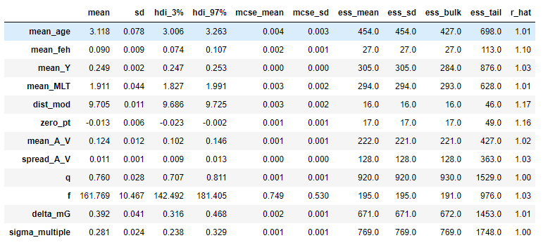
@grd349 The problem: The M67 HBM model has successfully make the sampler converge in (basically) all of the other cluster-wide parameters. The remaining two parameters that are still high in Rhat are distance modulus and Gaia parallax zero point offset. Even at 20000 tuning steps and 1000 sampling steps, they have 1.16 and 1.17 Rhats:

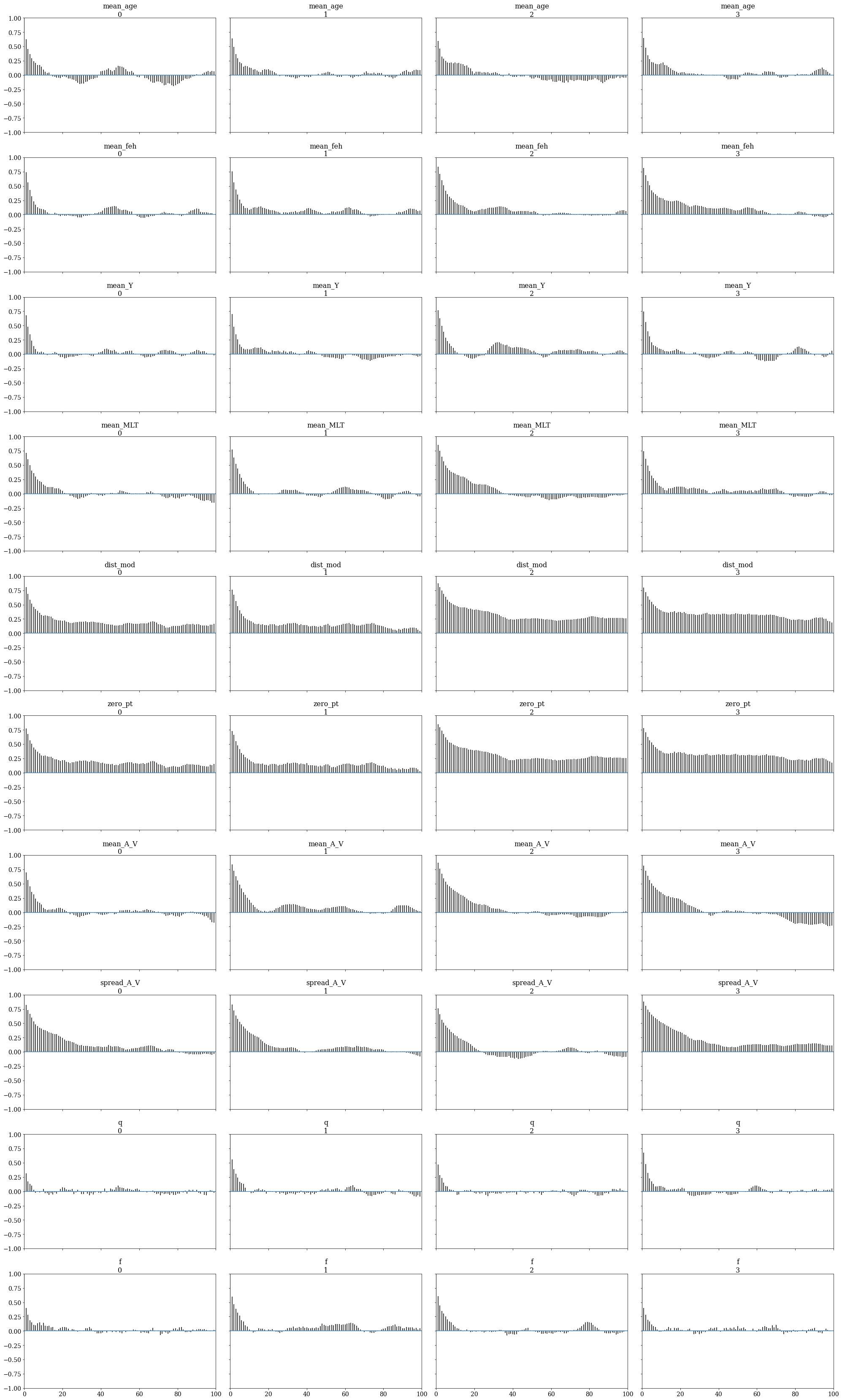
And high autocorrelation functions:

The current model:

[Av, dist_mod] = [0.11, 9.726]
M67_parallax = [1.1325,0.0011] #in milli arc seconds, from https://arxiv.org/pdf/1804.09378.pdf
M67_zero_point = [-82, 33] #in micro arc seconds, from https://ui.adsabs.harvard.edu/abs/2018ApJ...862...61S/abstract

model = pm.Model()
with model:
###### other model parts
    #distance and parallax
    dist_mod_ = pm.Normal('dist_mod', dist_mod, 1.0)
    true_parallax = pm.Deterministic('true_parallax', 10**(-dist_mod_/5-1)*1000)
    zero_pt = pm.Normal('zero_pt', M67_zero_point[0]/1000, M67_zero_point[1]/1000)
    obs_parallax = pm.Normal('obs_parallax', true_parallax+zero_pt, M67_parallax[1], observed=M67_parallax[0])

    #true observables
    true_mG = pm.Deterministic('true_mG', -2.5*T.log10(L)+Mbol-BCg+dist_mod_)
    true_Bp_Rp = pm.Deterministic('true_Bp_Rp', BCrp - BCbp)

######other model parts

(full model available in the next message)

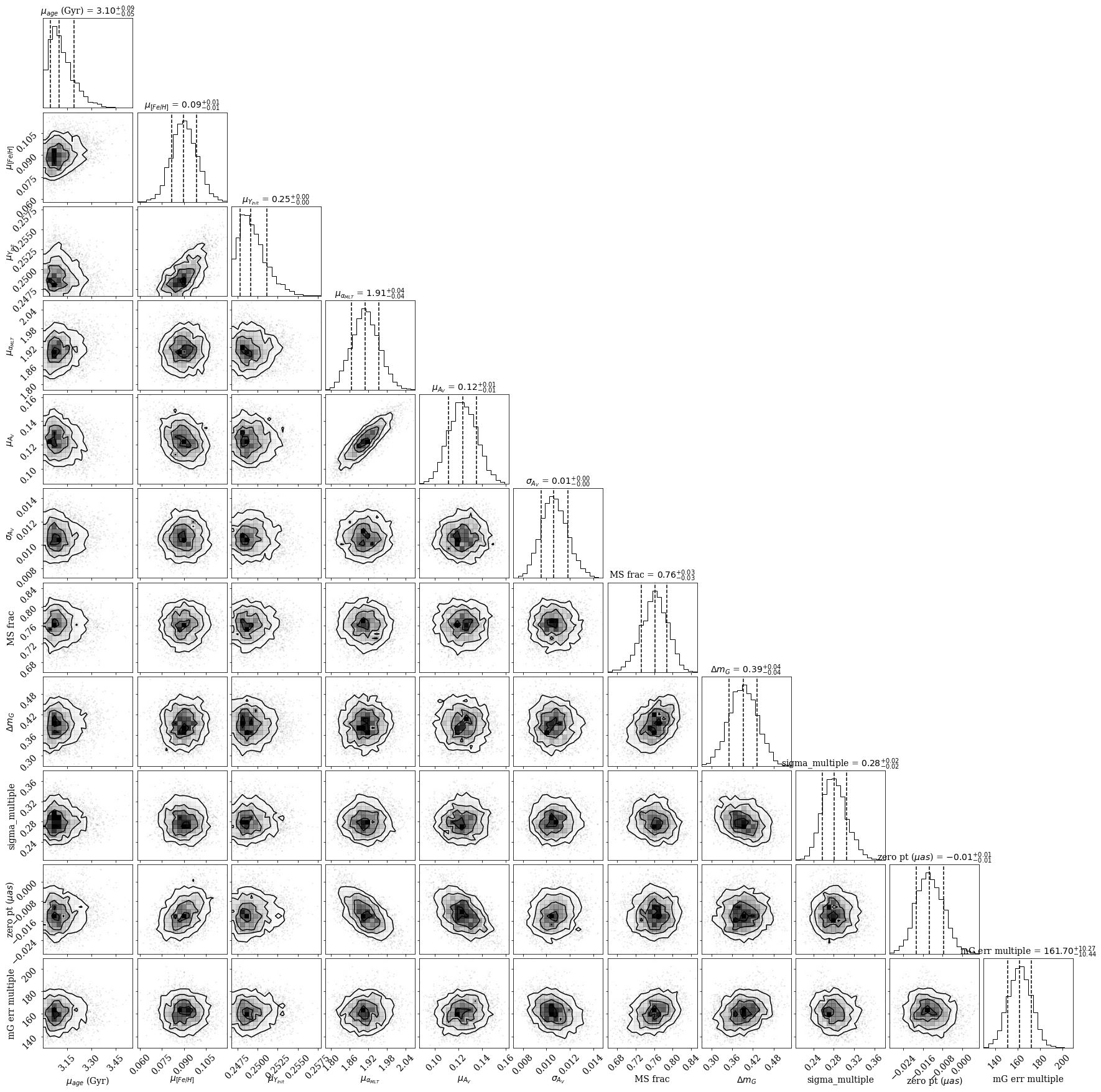
Corner plot to show correlations:

[HinLeung622]

full model:

model = pm.Model()
with model:

    #cluster-wide fundamentals
    Age_mu = pm.Deterministic('mean_age',pm.Beta('age_beta',2,2)*2+3)
    feh_mu = pm.Deterministic('mean_feh',pm.Beta('feh_beta',2,2)*0.3-0.15)
    Y_mu = pm.Deterministic('mean_Y',pm.Beta('Y_beta',2,2)*0.0334+0.2466)#0.24668 \pm 0.00007 is big bang nucleosynthesis fraction from Plank mission
    MLT_mu = pm.Deterministic('mean_MLT',pm.Beta('MLT_beta',10,10)*0.6+1.7)

    #per star fundamentals
    M = pm.Deterministic('mass', pm.Beta('mass_beta',1.1,1.1,shape=N)*(1.2-0.8)+0.8)
    Age = pm.Deterministic('age',T.ones(N)*Age_mu)
    feh = pm.Deterministic('feh',T.ones(N)*feh_mu)
    Y = pm.Deterministic('Y',T.ones(N)*Y_mu)
    MLT = pm.Deterministic('MLT',T.ones(N)*MLT_mu)

    #NN calculation
    obs = pm.Deterministic('obs',m1.manualPredict(T.log10([M, Age, 10**feh, Y, MLT])))

    #intermediate observables
    radius = pm.Deterministic('radius', 10**obs[0])
    Teff = pm.Deterministic('Teff', (10**obs[1])*5000)
    L = pm.Deterministic('L', (radius**2)*((Teff/Teff_sun)**4))
    logg = pm.Deterministic('logg', T.log10(100*constants.G.value*(M/radius**2)*(constants.M_sun.value/constants.R_sun.value**2)))
    true_s_feh = pm.Deterministic('true_s_feh', obs[3])
    obs_s_feh = pm.Normal('obs_s_feh', true_s_feh, M67['[Fe/H]_err'], observed=M67['[Fe/H]'])

    #extinction prior
    A_V_mu = pm.Deterministic('mean_A_V', pm.Beta('Av_beta',10,10)*0.2) # X & Y are 'sensible' values
    A_V_std = pm.Lognormal('spread_A_V', T.log(0.01), 0.1) # Different X & Y but still sensible
    A_V_ = pm.Normal('A_V_', 0, 1, shape=N) # an N(0, 1) dist to be scaled
    A_V = pm.Deterministic('A_V', A_V_ * A_V_std + A_V_mu)

    #second NN calculation
    BCs = pm.Deterministic('BCs', t1.manualPredict(T.as_tensor_variable([T.log10(Teff), logg, feh, A_V])))

    #BCs
    BCg = pm.Deterministic('BCg', BCs[5,:])
    BCbp = pm.Deterministic('BCbp', BCs[7,:])
    BCrp = pm.Deterministic('BCrp', BCs[8,:])

    #distance and parallax
    dist_mod_ = pm.Normal('dist_mod', dist_mod, 1.0)
    true_parallax = pm.Deterministic('true_parallax', 10**(-dist_mod_/5-1)*1000)
    zero_pt = pm.Normal('zero_pt', M67_zero_point[0]/1000, M67_zero_point[1]/1000)
    obs_parallax = pm.Normal('obs_parallax', true_parallax+zero_pt, M67_parallax[1], observed=M67_parallax[0])

    #true observables
    true_mG = pm.Deterministic('true_mG', -2.5*T.log10(L)+Mbol-BCg+dist_mod_)
    true_Bp_Rp = pm.Deterministic('true_Bp_Rp', BCrp - BCbp)

    #dealing with multiples
    q = pm.Beta('q', 1.1,1.1, testval=0.8)
    delta_mG = pm.Lognormal('delta_mG', T.log(0.3), 0.4)
    f = pm.Lognormal('f', T.log(10),0.7)
    sigma_multiple = pm.Lognormal('sigma_multiple', T.log(0.3), 0.3)
    dist_singular = pm.Normal.dist(0, np.mean(M67['g_mag_err'])*f)
    dist_multiple = pm.Normal.dist(-delta_mG, sigma_multiple)

    #obs observables
    obs_mG = pm.Mixture('obs_mG', w=[q, 1-q], comp_dists = [dist_singular, dist_multiple], \
                    observed=M67['g_mag'].values - true_mG)
    obs_Bp_Rp = pm.Normal('obs_Bp_Rp', mu=true_Bp_Rp, sigma=M67['Bp_Rp_err'], observed=M67['Bp_Rp'])

[HinLeung622]

@grd349 I just talked to a statistician in St Andrews in general terms about reducing autocorrelation (and hence Rhats) between samples in a dependent sampler, and he said that a rule of thumb would be to centralize a lot of the parameters by moving them to have roughly a mean of 0. I am applying this to both dist_mod and zero_pt parameters. They are the only two parameters left with normal distribution priors. So that part of the model now looks like this:

    #distance and parallax
    dist_mod_ = pm.Deterministic('dist_mod', dist_mod+pm.Normal('dist_mod_norm', 0, 1.0))
    true_parallax = pm.Deterministic('true_parallax', 10**(-dist_mod_/5-1)*1000)
    zero_pt_norm = pm.Normal('zero_pt_norm', 0, 1)
    zero_pt = pm.Deterministic('zero_pt', zero_pt_norm*M67_zero_point[1]/1000 + M67_zero_point[0]/1000)
    obs_parallax = pm.Normal('obs_parallax', true_parallax+zero_pt, M67_parallax[1], observed=M67_parallax[0])

[grd349]

@HinLeung622 - yes the parameterisation around zero might help.

I am also wondering if we can sacrifice out posterior estimate of the zero point offset and just propagate the offset and the uncertainty into our value of parallax and reduce the degeneracy. Do you know what I mean here, just proagate the uncertainty and offset on paper first and give the sampler one less thing to worry about.

[HinLeung622]

@grd349 You are saying to use external methods to estimate the zero pt error for the cluster outside of the HBM construct, then using that estimated value as a fixed input to the calculation within the HBM?

But how exactly does one do this when dist_mod and zero_pt are simply anti-correlated?

[grd349]

Because we have an estimate of the estimated parallax and the zero point offset, one can correct the estimated parallax for the offset on paper which produces a new 'corrected' parallax. Just use that value for the observed parallax and then there is no need to model the offset. Does that make sense?

[HinLeung622]

@grd349 Makes sense. Perhaps that will be the option if centralizing dist_mod and zero_pt priors do not help.

[HinLeung622]

@grd349 Results for using centralized priors on dist_mod and zero_pt: First, without centralized priors: Compared to with centralized priors: Both results are ran with the less aggressive Av priors, and 5000 tuning steps + 1000 sampling steps. Notably, the Rhats of the fundamentals, dist_mod and zero_pt all have lowered Rhats, while the other parameters have increased Rhats for some reason. Looking at the posterior traces, it seems the higher Rhats in the parameters mean Av and below are largely contributed by one single chain that deviated from the other 3. I am not sure if this result suggests an improvement in convergence thanks to centralized priors.

Anyhow, I will throw on many more tuning steps, maybe 50000, and 2000 sampling steps. This might take a week to run.

[HinLeung622]

@grd349 Turns out the maximum wall time on bluebear is 10 days/240 hours. It took 48 hours for 5000 tuning steps, so theoretically it would take 480 hours/20 days for 50000, which exceeds the max wall time. Any ideas?

[grd349]

We should focus on reparameterizing the model better so we don't need so many tuning steps. Did you have any luck with combining the parallax zero-point offset with the observed parallax into one observable value?

On Sat, 10 Oct 2020 at 17:09, HinLeung622 notifications@github.com wrote:

@grd349 https://github.com/grd349 Turns out the maximum wall time on bluebear is 10 days/240 hours. It took 48 hours for 5000 tuning steps, so theoretically it would take 480 hours/20 days for 50000, which exceeds the max wall time. Any ideas?

— You are receiving this because you were mentioned. Reply to this email directly, view it on GitHub https://github.com/Harry-Westwood/Y4-Project-InterNeuralStellar/issues/49#issuecomment-706572231, or unsubscribe https://github.com/notifications/unsubscribe-auth/ADQZOCJ5ZNDSVJJWUWAHBXTSKCBK3ANCNFSM4SHOGFGA .

[HinLeung622]

@grd349 Yeah, I had some success with the centralizing of the priors, it dropped Rhats of dist_mod and zero_pt from 1.8 to 1.5 on the same number of tuning and sampling steps (5000 and 1000). Look at the comparisons 2 replies above for details. Note that the enforcement of less informative priors on mean and spread Av resulted in the increase in Rhats in both of those runs above, compared to "better looking" runs I had in previous replies. This should have nothing to do with the centralizing of priors.

[HinLeung622]

@grd349 So I loaded bluebear with 4x more tuning steps (a version with 10x more is still running) and 2x more sampling steps for M67, with the less informative prior, which took 4 days x 36 cores to run: The large number of tuning steps pushed most of the Rhats down, except for again the dist_mod, zero_pt pair, but also feh, Y and spread_Av. Everything else looks sensible, including the estimated values for Y, feh, dist_mod, zero_pt, mean_Av and q (maybe not as much with the low age estimate but thats not the first time). Interestingly, the high Rhats do not destroy the corner plot: Strong covariance exist between: dist_mod and zero_pt (they vary directly with each other in the model) mean Av and MLT feh and [dist_mod and zero_pt] sigma Av vs mG_err_multiple (the larger the Av spread is, the smaller the width of the primary distribution in the mixture model has to be, to account for the width of the MS) And also a couple other weaker covariances, which some makes sense due to definition of the model.

I will report again if and when the larger tuning steps version finishes. It is strange how NGC188 is having good Rhats basically across the board with just 5k tuning steps while M67 is still struggling with 20k. Surely this could not be just due to the larger number of stars NGC188 has. I suspect there is some data falling into a lower likelihood region in one or more parameter for M67 that really gives the sampler a hard time, potentially through a multi-modal posterior.

[HinLeung622]

@grd349 I just found out about something when checking my sources: The numbers I use as the observed parallaxes for M67 and NGC188 are already zeropoint offset corrected, meaning I have been accounting for the offset twice. Since we want to do our own offset modelling, would it be more sensible to take the mean parallax of the members pulled from GAIA directly as the cluster parallax?

[HinLeung622]

@grd349 Correction: I read deeper into the GAIA paper that supplied the quoted parallax value for M67, and found that it did not account for the offset during the calculation of the overall parallax value of the whole cluster. This means that the value used previous is not zeropoint-corrected, meaning I have not been doing something wrong.

However, interestingly, the paper quotes literature values for dist mod, and shows 9.726 for M67. Converting that into parallax gives a value of 1.1345 mas, very close to their non-zeropoint-adjusted cluster mean parallax 1.1325. It is so close that the difference, supposedly to be the zeropoint offset, is only -0.002 mas, a magnitude lower than the GAIA's own rough estimate of -0.03mas, Oli's Kepler field estimate of -0.041mas and the paper Oli suggested that used EBs all over the sky to calibrate, which gave an estimate of -0.082mas. All of this is either: a. the quoted distance modulus value 9.726 from the GAIA paper is significantly wrong, which it might be since it came from isochrone fitting b. there is something very wrong with my calculations, or c. there is nearly no zeropoint offset for M67.

If the last possibility is the truth, we might be heavily skewing our dist_mod, and also other results by assuming the much larger -0.082mas offset. (eg. all current estimates of dist_mod have been ~ 9.5 after we opt to add zeropoint in quadrature instead of modelling it).

[grd349]

Yes - this is certainly something to think about. Maybe we need to do 3 different runs based on assumptions of different zero point offsets (i.e, no zero point, small zero point, large zero point).

On Thu, 5 Nov 2020 at 11:09, HinLeung622 notifications@github.com wrote:

@grd349 https://github.com/grd349 Correction: I read deeper into the GAIA paper that supplied the quoted parallax value for M67, and found that it did not account for the offset during the calculation of the overall parallax value of the whole cluster. This means that the value used previous is not zeropoint-corrected, meaning I have not been doing something wrong.

However, interestingly, the paper quotes literature values for dist mod, and shows 9.726 for M67. Converting that into parallax gives a value of 1.1345 mas, very close to their non-zeropoint-adjusted cluster mean parallax 1.1325. It is so close that the difference, supposedly to be the zeropoint offset, is only -0.002 mas, a magnitude lower than the GAIA's own rough estimate of -0.03mas, Oli's Kepler field estimate of -0.041mas and the paper Oli suggested that used EBs all over the sky to calibrate, which gave an estimate of -0.082mas. All of this is either: a. the quoted distance modulus value 9.726 from the GAIA paper is significantly wrong, which it might be since it came from isochrone fitting b. there is something very wrong with my calculations, or c. there is nearly no zeropoint offset for M67.

If the last possibility is the truth, we might be heavily skewing our dist_mod, and also other results by assuming the much larger -0.082mas offset. (eg. all current estimates of dist_mod have been ~ 9.5 after we opt to add zeropoint in quadrature instead of modelling it).

— You are receiving this because you were mentioned. Reply to this email directly, view it on GitHub https://github.com/Harry-Westwood/Y4-Project-InterNeuralStellar/issues/49#issuecomment-722309553, or unsubscribe https://github.com/notifications/unsubscribe-auth/ADQZOCJFWLDNN3NIDZPIASTSOKBWHANCNFSM4SHOGFGA .

[HinLeung622]

@grd349 Fair enough, it is unfortunate that we cannot model zeropoint at once.