IALSA / IALSA-2015-Portland

Hub to accompany IALSA 2015 workshop at Portland, OR, Feb 22-25, 2015
GNU General Public License v2.0
2 stars 0 forks source link

Guides for meta-analysis spreadsheet #180

Open andkov opened 7 years ago

andkov commented 7 years ago

Annotating meta-analysis

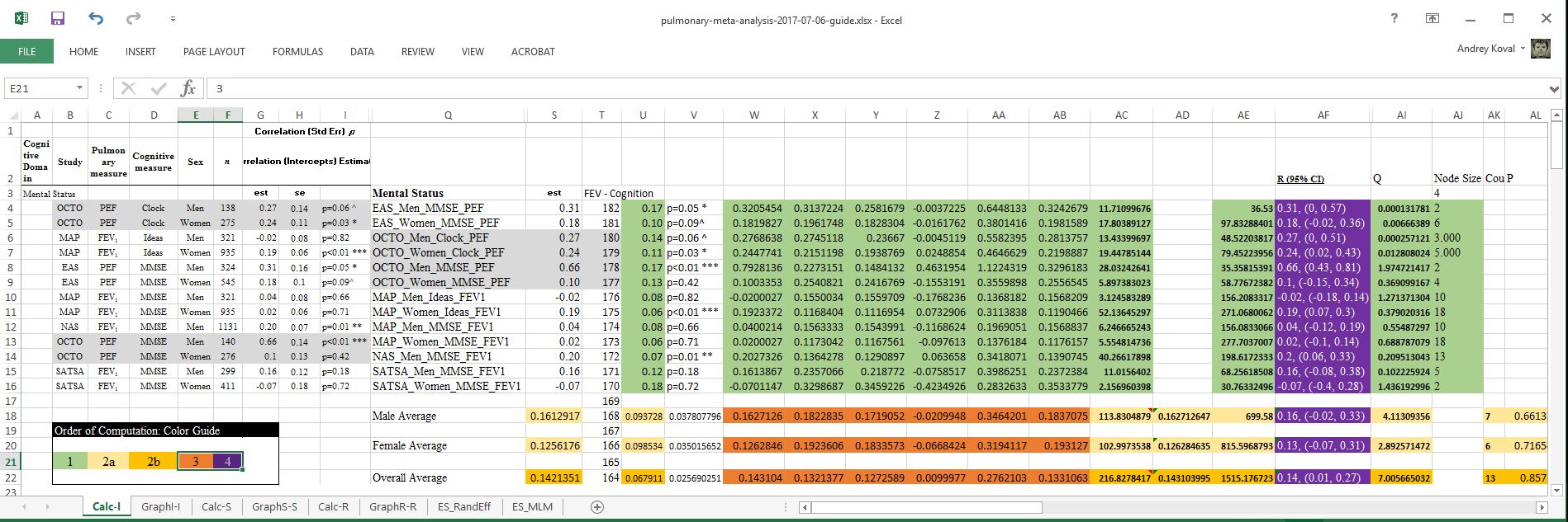
In pursuit of creating a transparent record of all computations undertaken during the implementation of meta-analysis and creation of the forest plots (see pulmonary-meta-analysis-2017-06-20.xlsx ), we have created a translation of the computations to be implemented in R and demonstrated this process with the R script ./sandbox/meta-analysis-demo.R and the excel companion guide pulmonary-meta-analysis-2017-07-06-guide.xlsx. The code and images to follow refer to contents of these files.

In the original spreadsheet, I have identified the cells that are actively engaged in producing the forest plot, located in the shaded area in the screenshot below

capture-1

The forest plot requires the following values: estimate, confidence intervals, and node size. The tricky part is to compute these values for subgroup and overall averages, which requires additional computaion.

capture-2

After cosmetic editing, we can tidy up the spreadsheet into the form that would easier to handle during annotation. capture-3

Finally, to demonstrate how the computations are carried out in R starting from the same data source, specific cells were colored to illustrate the sequence in which computations took place. The number of the sections (e.g. "1", "2a", "2b", "3") are referenced in the script ./sandbox/meta-analysis-demo.R . which details each set of operations.

This will be the main graphs referenced in this discussion.

andkov commented 7 years ago

Verifying the computations

You can follow along by running the following script:

# ---- load-packages -----------------------------------------------------------
library(tidyverse) 
# ---- load-data -------------------------------------------------------------
variable_names <- c("study_name","process_a", "process_b", "subgroup", "n", "est", "se")
proto <- list(
  row01 = c("OCTO"  ,"PEF"  ,"Clock" ,"Men"   ,138  , 0.27 ,0.14),
  row02 = c("OCTO"  ,"PEF"  ,"Clock" ,"Women" ,275  , 0.24 ,0.11),
  row03 = c("MAP"   ,"FEV1" ,"Ideas" ,"Men"   ,321  ,-0.02 ,0.08),
  row04 = c("MAP"   ,"FEV1" ,"Ideas" ,"Women" ,935  , 0.19 ,0.06),
  row05 = c("EAS"   ,"PEF"  ,"MMSE"  ,"Men"   ,324  , 0.31 ,0.16),
  row06 = c("EAS"   ,"PEF"  ,"MMSE"  ,"Women" ,545  , 0.18 ,0.10),
  row07 = c("MAP"   ,"FEV1" ,"MMSE"  ,"Men"   ,321  , 0.04 ,0.08),
  row08 = c("MAP"   ,"FEV1" ,"MMSE"  ,"Women" ,935  , 0.02 ,0.06),
  row09 = c("NAS"   ,"FEV1" ,"MMSE"  ,"Men"   ,1131 , 0.20 ,0.07),
  row10 = c("OCTO"  ,"PEF"  ,"MMSE"  ,"Men"   ,140  , 0.66 ,0.14),
  row11 = c("OCTO"  ,"PEF"  ,"MMSE"  ,"Women" ,276  , 0.10 ,0.13),
  row12 = c("SATSA" ,"FEV1" ,"MMSE"  ,"Men"   ,299  , 0.16 ,0.12),
  row13 = c("SATSA" ,"FEV1" ,"MMSE"  ,"Women" ,411  ,-0.07 ,0.18)
) %>%
  dplyr::bind_rows() %>%
  t() %>%
  tibble::as_tibble()
names(proto) <- variable_names
proto[,c("n","est","se")] <- sapply(proto[,c("n","est","se")], as.numeric)

This will recreate the data from the spreadsheet for the domain "Mental Status". This inputs all the data needed for analysis.

Question

I do not see where the spreadsheet utilized sample size. Are computations of the effect sized corrected for sample size? If yes, where?

Moving on

Operating on the object proto that contains estimates for the selected domain we compute the values in the green section:

# ---- tweak-data --------------------------------------------------------------
# green section: compute CI for observed estimates
ds1 <- proto %>%
  # compute  lower and upper limit of the 95% confidence (green section) for units
  dplyr::mutate(
    s  = est,                                             # Value of the estimate
    w  = log( (1 + s)/(1 - s) )/2,                        # ? w
    u  = (w * se)/ est,                                   # ? u - Value for standard error?
    ab = u * 1.96,                                        # ? ab
    aa = w + ab,                                          # ? aa
    z  = w - ab,                                          # ? z
    y  =     ( (exp(2*aa)-1) / (exp(2*aa)+1) ) - s,       # ? y
    x  = s - ( (exp(2*z)-1)  / (exp(2*z)+1)  )      ,     # ? x
    lo = -(x - s),                                        #  low 95% CI
    hi = y + s,                                           #  high 95% CI
    ac = abs( w/(u^2) ),                                  # ? ac
    ae = u^-2,                                            # ? ae  |  same as ag 
    ai = (z / 1.96)^2*ae,                                 # ? Q
    aj = ae / sum(ae) * 100                               # ? node size
  )
ds1 %>% dplyr::select_(.dots = c(variable_names,"s","u","w", "x","y","z","aa","ab","lo","hi"))

The output is better captured in a screenshot. capture-4

You can see that the values are identical to the values in the green section:

andkov commented 6 years ago

Compute group and overall averages

Now we compute group averages in light yellow

> # light yellow section: compute group averages
> ds2_group <- ds1 %>%
+   dplyr::group_by(subgroup) %>% # compute for each level off
+   dplyr::summarize(
+     ac = sum(ac),
+     ak = length(!is.na(u)),
+     ae = sum(ae),
+     ad = sum(ac)/sum(ae),                         
+     s  = (exp(2*ad)   - 1) / (exp(2*ad)   + 1),
+     u  = 1/sqrt(ad*ae),
+     ai = sum(ai)
+   )
> ds2_group
# A tibble: 2 × 8
  subgroup       ac    ak       ae        ad         s          u       ai
     <chr>    <dbl> <int>    <dbl>     <dbl>     <dbl>      <dbl>    <dbl>
1      Men 113.8305     7 699.5798 0.1627126 0.1612917 0.09372829 4.113094
2    Women 102.9974     6 815.5969 0.1262846 0.1256176 0.09853419 2.892571

And the overall averages in dark yellow :

# dark yellow section : computing overall averages
ds2_overall <- ds1 %>%
  # dplyr::group_by(subgroup) %>% # notice that this is turned OFF now
  dplyr::summarize(
    ad = sum(ac)/sum(ae),                          # ? ad
    ak = length(!is.na(u)),
    ac = sum(ac),
    ae = sum(ae),
    s  = (exp(2*ad)   - 1) / (exp(2*ad)   + 1), # ? s
    u  = 1/sqrt(ad*ae),
    ai = sum(ai),
    al = pchisq(ai,   df = ak   - 1, lower.tail = FALSE)
  ) %>%
  dplyr::mutate(subgroup = "Overall") %>%
  dplyr::select(subgroup, dplyr::everything())
ds2_overall %>%  dplyr::select_(.dots = c("subgroup","s","u", "ac","ae","ai", "ak","al"))
> ds2_overall %>%  dplyr::select_(.dots = c("subgroup","s","u", "ac","ae","ai", "ak","al"))
# A tibble: 1 × 8
  subgroup         s          u       ac       ae       ai    ak       al
     <chr>     <dbl>      <dbl>    <dbl>    <dbl>    <dbl> <int>    <dbl>
1  Overall 0.1421351 0.06791137 216.8278 1515.177 7.005665    13 0.857239

Now we merges files containing group and overall averages:

# red section : combine and compute values of CI for derived averages
ds3 <- dplyr::bind_rows(ds2_group, ds2_overall) %>%
  dplyr::mutate(
    w  = log( (1 + s)/(1 - s) )/2,                        # ? w
    ab = u * 1.96,                                        # ? ab
    aa = w + ab,                                          # ? aa
    z  = w - ab,                                          # ? z
    y  =     ( (exp(2*aa)-1) / (exp(2*aa)+1) ) - s,   # ? y
    x  = s - ( (exp(2*z)-1)  / (exp(2*z)+1)  )      ,   # ? x
    lo = -(x - s),                                      #  low 95% CI
    hi = y + s                                         #  high 95% CI
   ) 
> ds3 %>%  dplyr::select_(.dots = c("subgroup","s","u", "ac","ae","ai", "ak","al"))
# A tibble: 3 × 8
  subgroup         s          u       ac        ae       ai    ak        al
     <chr>     <dbl>      <dbl>    <dbl>     <dbl>    <dbl> <int>     <dbl>
1      Men 0.1612917 0.09372829 113.8305  699.5798 4.113094     7 0.6613749
2    Women 0.1256176 0.09853419 102.9974  815.5969 2.892571     6 0.7165438
3  Overall 0.1421351 0.06791137 216.8278 1515.1767 7.005665    13 0.8572390

Finally, we contruct the display values for est( low, high) dense values:

# purple section
ds4 <- ds1 %>%
  # dplyr::select(-ac,-ae) %>%
  dplyr::bind_rows(ds3) %>%
  dplyr::mutate(
    af = sprintf("%.2f(%.2f,%.2f)", s, lo, hi)          #  estimate(low, high)
  )
ds4 %>%
  dplyr::select_(.dots = c(variable_names,"af","ai","aj","ak","al" ))

capture-5