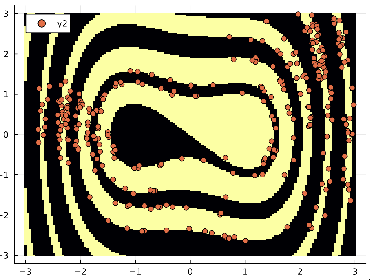
What's the code for the second figure? And which of the three options does it implement? Option (2) ?
Open awage opened 1 year ago
What's the code for the second figure? And which of the three options does it implement? Option (2) ?
I post the code here, the option (2) with the hit and run algorithm. I am not sure I implemented it correctly. It is a first attempt. It is not optimal since the purpose of the code was to evaluate the basin entropy of the boundary. But it is the same principle for the exploration of the boundary:
using Plots
using OrdinaryDiffEq
using Attractors
using Statistics

@inline @inbounds function duffing(u, p, t)
    d = p[1]; F = p[2]; omega = p[3]
    du1 = u[2]
    du2 = -d*u[2] + u[1] - u[1]^3 + F*sin(omega*t)
    return SVector{2}(du1, du2)
end

function get_basins_nfo(F, ω, grid)
    ds = StroboscopicMap(2π/ω, duffing, rand(2), [0.15, F, ω], diffeq = (;reltol = 1e-8, alg = Vern9()))
    mapper = AttractorsViaRecurrences(ds, grid; sparse = true,
        store_once_per_cell = true,
        mx_chk_loc_att = 10000, mx_chk_safety = Int(1e7), show_progress = true)
    return mapper
end

function multi_threaded_basins(mapper, u0s)
    nthreads = Threads.nthreads()
    map_v = [deepcopy(mapper) for i in 1:nthreads]
    bas = zeros(Int16, length(u0s))
    Threads.@threads for j in 1:length(u0s)
        bas[j] = map_v[Threads.threadid()](u0s[j])
    end
    return bas
end

function hit_and_run_random_walk(F, ω, mapper, Nw = 1000)
    # Dummy grid for computations
    xg = yg = range(-3,3,length=10)
    Mx = maximum(xg)
    mx = minimum(xg)
    My = maximum(yg)
    my = minimum(yg)
    # Generate N random samples in a radius ϵ centered at a random point u1 in [xg, yg]
    # First uniform sampler:
    ε = 0.1; N = 100; #Na = length(unique(basins))
    s_v = zeros(Nw)
    # initial condition.
    u1 = [mx + (Mx - mx)*rand(), my + (My - my)*rand()]
    uv = Vector{typeof(u1)}()
    for k in 1:Nw
        uc = _hit_and_run(4*ε, u1, mx, Mx, my, My)
        s  = _get_ball_entropy(ε, N, uc, mapper)
        u1 = _rejection_filter(s, uc, u1)
                if s > 0
                    push!(uv, u1)
                end
        s_v[k] = s
    end
    return s_v, uv
end

function _rejection_filter(s, uc, u1)
    # Rejection filter
    if s == 0.
        # if we are in the interior, move to uc with probability p (arbitrary for now)
        return (rand() < 0.2 ? uc : u1)
    else
        # accept candidate if s > 0
        return uc
    end
end

function _hit_and_run(λ, u1, mx, Mx, my, My)
    reject = true;
    while reject
        # choice of a random direction on the circle:
        θ = rand()*2π
        rd = [cos(θ), sin(θ)]
        uc = u1 .+ rd*λ
        # check bounds
        if (mx < uc[1] < Mx) && (my < uc[2] < My)
            reject = false
            return uc
        end
    end
end

function _get_ball_entropy(ε, N, u1, mapper)
    u2s = [u1 + ε*[rand()-0.5, rand()-0.5] for k in 1:N]
    bsn = multi_threaded_basins(mapper, u2s)
    @show p = _box_entropy(bsn)
    return p
end

function _box_entropy(box_values)
    h = 0.
    for (k,v) in enumerate(unique(box_values))
        p = count( x -> (x == v), box_values)/length(box_values)
        h += p*log(1/p)
    end
    return h
end

# F = 0.128; ω = 1.106
F = 0.1; ω = 0.2
xg = yg = range(-3,3,length = 150)
mapper = get_basins_nfo(F, ω, (xg, yg));

@time b1, v = hit_and_run_random_walk(F, ω, mapper, 1000)

v = Dataset(v)
b,a = basins_of_attraction(mapper, (xg,yg))
heatmap(xg,yg, b')
plot!(v[:,1],v[:,2], seriestype = :scatter)
im guessing we could actually make a paper if we come up with an algorithm to find the basin. However, isn't this also what the saddle straddle does in #118 ? Or it is not generic enough to apply to "any" basin boundary?
There is no automated algorithm in DynamicalSystems.jl to explore the boundary between two basins. Here are some ideas from simple to difficult:
There is an enormous amount of works in stochastic search (MCMC, Metropolis-Hasting, hit-and-run ...). And there very nice Julia packages that covers the subject.
I post here a naive attempt with the hit and run algorithm for the Duffing oscillator.
Smooth boundaries are harder to find.