Closed troyrock closed 3 years ago
Hi -- happy to help.
The way you would do that with AbstractGPs.jl / Stheno.jl is something like:
x = range(0.0, 1.0; length=1_000)
f = GP(SEKernel() ∘ ScaleTransform(1 / 0.2))
sampleplot(f(x); samples=10)
(I might be off by a factor of two with the length scale or something)
Internally, kernelmatrix(SEKernel() ∘ ScaleTransform(1 / 0.2), x)
will be called, which is what I think you're after with K(x)
.
I'm trying it now (sorry about the delay and thank you for the response!) What does the little circle mean and how do I type it in? Right now I cut and pasted it...
I am getting an error: MethodError: no method matching plot(::AbstractGPs.SamplePlot{StepRangeLen{Float64, Base.TwicePrecision{Float64}, Base.TwicePrecision{Float64}}, AbstractGPs.FiniteGP{GP{AbstractGPs.ZeroMean{Float64}, TransformedKernel{SqExponentialKernel{Distances.Euclidean}, ScaleTransform{Float64}}}, StepRangeLen{Float64, Base.TwicePrecision{Float64}, Base.TwicePrecision{Float64}}, Diagonal{Float64, FillArrays.Fill{Float64, 1, Tuple{Base.OneTo{Int64}}}}}}; samples=10)
collect(f(x))
gives me a similar error: ERROR: MethodError: no method matching iterate(::AbstractGPs.FiniteGP{GP{AbstractGPs.ZeroMean{Float64}, TransformedKernel{SqExponentialKernel{Distances.Euclidean}, ScaleTransform{Float64}}}, StepRangeLen{Float64, Base.TwicePrecision{Float64}, Base.TwicePrecision{Float64}}, Diagonal{Float64, FillArrays.Fill{Float64, 1, Tuple{Base.OneTo{Int64}}}}})
What does the little circle mean and how do I type it in?
If you type \circ
and press tab at the REPL, you'll get the symbol. It's the composition operator.
Regarding sampleplot
, you'll need to using Plots
first (sorry, forgot about that). Also, you'll actually want to use
sampleplot(f(x, 1e-12); samples=10)
to make sure that the covariance matrix constructed under the hood is positive definite.
Also, you'll actually want to use
sampleplot(f(x, 1e-12); samples=10)
to make sure that the covariance matrix constructed under the hood is positive definite.
Alternatively, you can use
sampleplot(x, f; samples=10)
which takes care of this automatically.
This worked! Thank you.
x = range(0.0, 1.0; length=1000)
f = GP(SEKernel() ∘ ScaleTransform(1/l))
k = kernelmatrix(SEKernel() ∘ ScaleTransform(1/l), x)
l = cholesky(k+Diagonal(1e-13*ones(1000))).L
u = rand(1000, 10)
r = transpose(l * u)
p = plot(r[1,:])
for num in range(2,length=9)
plot!(p, r[num,:])
end
p
I can not figure out what I'm doing wrong here but I can't seem to duplicate the results by doing it manually. (I had hoped to be able to get the "function" values of the things plotted by sampleplot by looking at the code but trying to follow what is happening with @recipe
and all the levels of indirection made my head spin.) Any help would be appreciated.
It's not clear which lenghtscale l
you used, is it the same as above? More importantly though, you have to sample u
with randn
(rand
samples uniformly at random from the unit interval), ie. you have to use u = randn(1000, 10)
.
The simplest thing to do is just
rand(f(x, 1e-12), 10)
You can find the code here: https://github.com/JuliaGaussianProcesses/AbstractGPs.jl/blob/9b14c286e5885c2e94edf5bc3502347126b23276/src/abstract_gp/finite_gp.jl#L227
edit: FWIW, I also find it hard to follow what's going on inside plotting recipes, so you're not alone there!
Thank you very much! Hopefully as I learn more, I'll be able to help others as well.
I've been trying to figure out how to utilize Stheno.jl to duplicate some code I found in python. I'm new to kernels and how they are used so don't hesitate to explain what I'm not understanding. The python code uses the squared exponential kernel (Radial Basis Functions) to produce n random but smooth functions:
When I plot the results I get plots that look like the following for n=10:
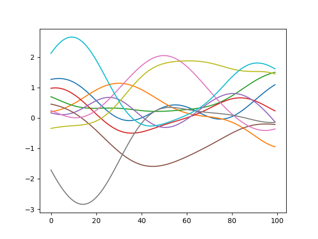
Unfortunately I get stuck early on when I want to produce the radial basis functions of x (
k=K(x)
). Any help is appreciated.