Contributed Examples

[shashi]

We should probably find a better way to collect examples. Meanwhile, let's use this issue to show off cool things you create with Interact. Code snippets, nbviewer / github links are all welcome.

Here's something to start this off :)

# (phantom) particles in a box

using Reactive, Interact
using Color, Compose

box(x) = let i = floor(x)
    i%2==0 ? x-i : 1+i-x
end

colors = distinguishable_colors(10, lchoices=[82.])

dots(points) = [(context(p[1], p[2], .05, .05), fill(colors[i%10+1]), circle())
    for (i, p) in enumerate(points)]

@manipulate for t=timestamp(fps(30)), add=button("Add particle"),
    velocities = foldl((x,y) -> push!(x, rand(2)), Any[rand(2)], add)

    compose(context(),
            dots([map(v -> box(v*t[1]), (vx, vy)) for (vx, vy) in velocities])...)
end

[stevengj]

using Color, Compose, Interact
const colors = distinguishable_colors(6)
function sierpinski(n, colorindex=1)
    if n == 0
        compose(context(), circle(0.5,0.5,0.5), fill(colors[colorindex]))
    else
        colorindex = colorindex % length(colors) + 1
        t1 = sierpinski(n - 1, colorindex)
        colorindex = colorindex % length(colors) + 1
        t2 = sierpinski(n - 1, colorindex)
        colorindex = colorindex % length(colors) + 1
        t3 = sierpinski(n - 1, colorindex)
        compose(context(),
                (context(1/4,   0, 1/2, 1/2), t1),
                (context(  0, 1/2, 1/2, 1/2), t2),
                (context(1/2, 1/2, 1/2, 1/2), t3))
    end
end

@manipulate for n = 1:8
    sierpinski(n)
end

[stevengj]

http://nbviewer.ipython.org/github/stevengj/Julia-EuroSciPy14/blob/master/Interactive%20Widgets.ipynb

[stevengj]

@shashi, your example above yields

`start` has no method matching start(::Button{Nothing})
while loading In[2], in expression starting on line 13

 in mapfoldl at reduce.jl:67
 in foldl at reduce.jl:84

for me.

[stevengj]

Here's an example I used yesterday to explain the convergence of Newton's method for sqrt(2) to a student:

using Interact

# n steps of Newton iteration for sqrt(a), starting at x
function newton(a, x, n)
    for i = 1:n
        x = 0.5 * (x + a/x)
    end
    return x
end

# output x as HTML, with digits matching x0 printed in bold
function matchdigits(x::Number, x0::Number)
    s = string(x)
    s0 = string(x0)
    buf = IOBuffer()
    matches = true
    i = 0
    print(buf, "<b>")
    while (i += 1) <= length(s)
        i % 70 == 0 && print(buf, "<br>")
        if matches && i <= length(s0) && isdigit(s[i])
            if s[i] == s0[i]
                print(buf, s[i])
                continue
            end
            print(buf, "</b>")
            matches = false
        end
        print(buf, s[i])
    end
    matches && print(buf, "</b>")
    html(takebuf_string(buf))
end

set_bigfloat_precision(1024)
sqrt2 = sqrt(big(2))
@manipulate for n in slider(0:9, value=0, label="number of Newton steps:")
     matchdigits(newton(big(2), 2, n), sqrt2)
end

[shashi]

@stevengj I was on master branch of Reactive and just about to tag a new version, Pkg.update() should fix it now. Really like the Newton's square root example! And the EuroPy talk notebooks are neat! I'm waiting to watch the video.

[dcjones]

Playing more with color palettes. This makes me want to paint my apartment.

using Color, Reactive, Interact

@manipulate for n in 1:12,
                hmin in 1:5:360, hmax in 1:5:360,
                cmin in 1:100, cmax in 1:100,
                lmin in 1:100, lmax in 1:100
    distinguishable_colors(n, hchoices=linspace(hmin, hmax, 30),
                           cchoices=linspace(cmin, cmax, 20),
                           lchoices=linspace(lmin, lmax, 20))
end

[vchuravy]

For me the best thing is the simplicity of making things like this happen:

using Interact, Gadfly, Distributions

@manipulate for α in 1:100, β = 1:100
    plot(x -> pdf(Beta(α, β), x), 0, 1)
end

[shashi]

@vchuravy that's a much nicer example than the one in the example notebook right now. Will steal it for the next release ;)

[shashi]

using AudioIO, Interact, Gadfly
s1 = SinOsc(220)
s2 = SinOsc(220)
@manipulate for f1=100:880, f2 = 110:880
    s1.renderer.freq = f1
    s2.renderer.freq = f2
    plot(t->sin(f1*2pi*t) + sin(f2*2pi*t), 0, 2pi)
end
play(s1)
play(s2)

cc ssfrr/AudioIO.jl#27

[ssfrr]

@shashi That is a super awesome example. This opens up a lot of new doors and is definitely encouraging me to make Interact a first-class citizen in the AudioIO world.

[shashi]

@ssfrr nice! I'm more for keeping keeping AudioIO and Interact orthogonal and making them work well together rather than inside one another though ;)

[shashi]

"In Julia and perhaps your language, there are knobs that make it even easier to watch the algorithm in action."

@alanedelman's illustration of how matrix multiplication happens with different loop orders.

function matmul_ijk(a,b,stop)
    step=0
    n=size(a,1)
    c=zeros(a)
    for i=1:n, j=1:n, k=1:n  
        if step==stop;  return(c); end
        c[i,j] +=  a[i,k] * b[k,j]
        step+=1
    end
    c
end

function matmul_kji(a,b,stop)
    step=0
    n=size(a,1)
    c=zeros(a)
    for k=1:n, j=1:n, i=1:n  
        if step==stop;  return(c); end
        c[i,j] +=  a[i,k] * b[k,j]
        step+=1
    end
    c
end

n=10
o=int(ones(n,n))
@manipulate for stop=0:n^3
    matmul_ijk(o,o,stop)
end

n=10
o=int(ones(n,n))
@manipulate for stop=0:n^3
    matmul_kji(o,o,stop)
end

[vchuravy]

I found this recently: @dlfivefifty https://github.com/dlfivefifty/ApproxFun.jl/blob/master/examples/Mainpulate%20Helmholtz.ipynb Which solves the Helmholtz equation and manipulates the parameters via Interact

[catawbasam]

filter iris DataFrame by species

using Reactive, Interact
using DataFrames

using RDatasets
iris = dataset("datasets", "iris")
speciespool = iris[:Species].pool

@manipulate for species=speciespool
    iris[ iris[:Species] .==species , :]
end

[jiahao]

Here is an example of code to draw parallel prefix trees. The @manipulate call at the very end allows you to play with how the compute tree varies with the number of processors.

using Compose, Interact

#Brent-Kung parallel prefix
function prefix!(y, +)
    l=length(y)
    k=iceil(log2(l))
    @inbounds for j=1:k, i=2^j:2^j:min(l, 2^k)              #"reduce"
        y[i] = y[i-2^(j-1)] + y[i]
    end
    @inbounds for j=(k-1):-1:1, i=3*2^(j-1):2^j:min(l, 2^k) #"broadcast"
        y[i] = y[i-2^(j-1)] + y[i]
    end
    y
end

# Instrumentation

import Base: getindex, setindex!, length

type AccessArray
    length :: Int
    read :: Vector
    history :: Vector
    AccessArray(length, read={}, history={})=new(length, read, history)
end

length(A::AccessArray)=A.length

function getindex(A::AccessArray, i)
    push!(A.read, i)
    nothing
end

function setindex!(A::AccessArray, x, i)
    push!(A.history, (A.read, {i}))
    A.read = {}
end

# Renderer
type gate
    ins :: Vector
    outs:: Vector
end

function render(G::gate, x₁, y₁, y₀; rᵢ=0.1, rₒ=0.25)
    ipoints = [(i, y₀+rᵢ) for i in G.ins]
    opoints = [(i, y₀+0.5) for i in G.outs]
    igates  = [circle(i..., rᵢ) for i in ipoints]
    ogates  = [circle(i..., rₒ) for i in opoints]
    lines = [line([i, j]) for i in ipoints, j in opoints]
    compose(context(units=UnitBox(0.5,0,x₁,y₁+1)),
        compose(context(), stroke("black"), fill("white"),
            igates..., ogates...),
        compose(context(), linewidth(0.3mm), stroke("black"),
            lines...))
end

function render(A::AccessArray)
    #Scan to find maximum depth
    olast = depth = 0
    for y in A.history
        (any(y[1] .≤ olast)) && (depth += 1)
        olast = maximum(y[2])
    end
    maxdepth = depth

    olast = depth = 0
    C = {}
    for y in A.history
        (any(y[1] .≤ olast)) && (depth += 1)
        push!(C, render(gate(y...), A.length, maxdepth, depth))
        olast = maximum(y[2])
    end

    push!(C, compose(context(units=UnitBox(0.5,0,A.length,1)),
      [line([(i,0), (i,1)]) for i=1:A.length]...,
      linewidth(0.1mm), stroke("grey")))
    compose(context(), C...)
end

#The actual call to manipulate
@manipulate for np=1:100
    render(prefix!(AccessArray(np),+))
end

Observe that the depth of the tree grows by one at powers of two and 3 x powers of two.

[Edit: fixed link]

[shashi]

Here is a bouncing ball that works using Patchwork

using Reactive, Interact, Patchwork.SVG
@manipulate for t=timestamp(fps(30))
    y = (1-abs(cos(2t[1])))*.9
    svg(circle(cx=.5, cy=y, r=.1, fill=:tomato),
        viewBox="0 0 1 1",  height="4in", width="4in")
end

it simply constructs a representation of the SVG to be drawn, then upon every update to t, diffs the next representation with the current one to calculate a set of patches and sends only the patches to the browser. The browser then applies the patch to the appropriate DOM elements. In this case, only the <circle> element's cy property is updated on each tick.

In most cases it reduces the number of bytes to be transferred.

Another (probably more important) advantage of the diff-patching approach is that any other state associated with the DOM elements is preserved after an update. For example:

using Patchwork.HTML5, Interact
@manipulate for n = slider(1:20)
    ul([li(input(value=i)) for i=1:n])
end

Here n text input boxes are produced. You may type into these boxes, update the slider and still have the text in the text boxes remain after the update -- the update only causes a certain number of input elements to be added or removed from the end of the existing list.

I am hoping this will provide a starting point to truly interactive visualizations, not just limited to sliders, checkboxes and such. Think compose graphics that update themselves when you click or drag elements in them (ref #38)

[stevengj]

Here's an example I used in class yesterday (see notebook) to illustrate Newton's method in the complex plane:

using Interact, PyPlot

# Newton's method to solve x^k = a, starting with x, for n iterations or until tol is reached
function newtonroot(k, a, n, x, tol=1e-3)
    tol² = tol*tol
    for i = 1:n
        oldx = x
        x = ((k-1)*x + a/x^(k-1))/k
        # to speed things up, stop early if x changes by < tol
        if abs2(x - oldx) < tol²
            break
        end
    end
    return x
end

# convert a k-th root of unity, from initial guess z, into a phase angle
function rootangle(k, z)
    θ = angle(newtonroot(k, 1, 25, z))/pi
    θ = θ < -0.95 ? 1.0 : θ # eliminate ±π oscillations from branch cut
    return θ
end
rootangles(k, X, Y) = Float64[rootangle(k, x+im*y) for y in Y, x in X]   

f = figure()
ξ = linspace(-2,2,600)
@manipulate for k in 2:10
    withfig(f) do
        imshow(rootangles(k, ξ, ξ), extent=(-2,2,-2,2)) # imshow is faster than pcolor
        xlabel(L"\Re z")
        ylabel(L"\Im z")
        title("Basins of attraction for $k-th roots of unity")
        colorbar(label="phase angle of root / π")
        roots = exp(2*π*im*[1:k]/k)
        plot(real(roots), imag(roots), "ko")
    end
end

[jiahao]

Here's one for visualizing the singular value decomposition from this IJulia notebook with Gadfly:

using Color
using Gadfly
using Interact

#Plot a given left and right singular vector and also its position in the spectrum of singular values
function plotsvd(S::Base.LinAlg.SVD, i::Int)
    m = size(S[:U], 1) #Reconstruct dimensions of matrix that was SVDed
    n = size(S[:V], 2)
    ns= size(S[:S], 1)

    leftcolors = reverse(colormap("Reds", ns+1))
    rightcolors = reverse(colormap("Blues", ns+1))
    hstack(
        #Left singular vector
        plot(x=1:m, y=sub(S[:U],:,i), Geom.line,
            Theme(default_color=leftcolors[i]),
            Guide.xlabel("Time"), Guide.ylabel(""),
            Guide.title("U[$i]")),

        #Singular values
        plot(x=1:ns, y=S[:S], Geom.point, Geom.line, 
            xintercept = [i], Geom.vline,
            Theme(default_color=color("black")),
            Guide.xlabel("Rank"), Guide.ylabel(""),
            Guide.title("σ[$i] = $(S[:S][i])")),

        #Right singular vector
        plot(x=1:n, y=sub(S[:Vt],i,:), Geom.bar,
            Theme(default_color=rightcolors[i]),
            Guide.xlabel("Data id"), Guide.ylabel(""),
            Guide.title("V[$i]")),
    )
end

S = svdfact(data)
set_default_plot_size(1000px, 400px)
@manipulate for i=1:size(S[:S], 1)
    plotsvd(S, i)
end

[Ken-B]

Here's a simple timer with reset button:

using Interact, Reactive
timer = togglebutton("timer")
reset = button("reset", value = :reset)
map(display, [timer,reset])

dt = .5
sig = merge(keepwhen(signal(timer), 0, every(float(dt))), signal(reset))
foldl((acc,val) -> val == :reset ? 0 : acc + dt, 0., sig)

[ma-laforge]

Use Interact to get feel for how gain & pole/zero locations affect stability.

https://github.com/ma-laforge/InspectDR.jl/blob/master/notebook/2_interact.ipynb

(Sorry, need to check out master branch of InspectDR.jl to test notebook at the moment).

[ma-laforge]

A slightly more complex example examining PLL (phase locked loop) characteristics:

https://github.com/ma-laforge/InspectDR.jl/blob/master/notebook/3_pllstab.ipynb (Again, need to check out master branch of InspectDR.jl to test out at the moment).

[korsbo]

My work largely consists of playing around with systems of differential equations. I have thus found it useful to create a function which allows me to interactively change parameter values (etc.) and plot the resulting simulation.

This demo forgoes the @manipulate macro in favour of map() combined with signal().

using Interact
using DifferentialEquations
using Latexify
using Plots 
gr()

"""
A function which simulates and plots an ODE. 

The system is first equilibrated for an input value of 1.
The plotted dynamics is the relaxation of the system after the input is changed to 10.
"""
function plotODE(ode, parameters, plotvars)
    parameters[1] = 1.
    u0 = fill(1., length(ode.syms))
    ssprob = SteadyStateProblem(ode, u0, parameters)
    u0 = solve(ssprob).u

    tspan = (0.,10.)
    parameters[1] = 10.
    prob = ODEProblem(ode, u0, tspan, parameters)
    sol = solve(prob, solver=Rosenbrock23())

    plot(sol, vars=plotvars, xlabel="Time", ylabel="Concentration", ylims=[0.,-Inf])
end

"""
Automatically generate sliders for all the ODE's parameters and map the results 
to the plotODE function.
"""
function interactivePlot(ode)
    display(latexalign(ode))
    params = [selection_slider(signif.(logspace(-2,2,101), 3), label=latexify(p)) 
        for p in ode.params]
    plotvars = selection(ode.syms, multi=true)

    display(hbox(vbox(params[2:end]...), plotvars))

    map((x...)->plotODE(ode, collect(x[1:end-1]), x[end]), 
        signal.(params)..., signal(plotvars))
end

"""
Define some ODEs
"""
ode1 = @ode_def NegativeFeedback begin
    dx = r_x * (e_x * input * y - x)
    dy = r_y * (e_y / x - y)
end input r_x e_x r_y e_y 

ode2 = @ode_def IncoherentFeedForward begin
    dx = r_x * (e_x * input - x)
    dy = r_y * (e_y * input / x - y)
end input r_x e_x r_y e_y

ode3 = @reaction_network InducedDegradation begin
    (input*r_bind, r_unbind), X_free ↔ X_bound
    (p_free, d_free), 0 ↔ X_free 
    d_bound, X_bound --> 0 
end input r_bind r_unbind p_free d_free d_bound

This will automatically generate a small interface to whatever ParameterizedFunction or ReactionNetwork you throw at it:

[edit] Update for API change of DifferentialEquations 4+

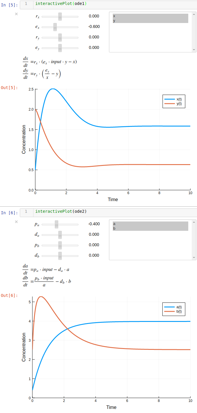
[asinghvi17]

Updated version of @korsbo's example compatible with Julia 1.0.2, Interact v0.9.0, DifferentialEquations v5.3.1:

Importing required packages:

using Interact, 
      DifferentialEquations, 
      Latexify, 
      Plots,
      WebIO

Function definitions

"""
A function which simulates and plots an ODE. 

The system is first equilibrated for an input value of 1.
The plotted dynamics is the relaxation of the system after the input is changed to 10.
"""
function plotODE(ode, parameters, plotvars, initcond)
    tspan = (0.,100.)
    prob = ODEProblem(ode, initcond, tspan, parameters)
    sol = solve(prob)

    plot(
        plot(sol, vars=(:v, :w), xlabel="v", ylabel="w", title="Phase plot"), # make the phase plot
        plot(sol, vars=(:t, :v, :w), legend=:none, title="Phase(t)"),   # plot phase vs time
        plot(sol, title="FHN solution", xlabel="Time"), # plot the solution versus time
        layout=@layout [ a b
                          c  ]
        )

end

"""
Automatically generate sliders for all the ODE's parameters and map the results 
to the plotODE function.
"""
function interactivePlot(ode, initcond)
    display(latexalign(ode))
    params = [slider(round.(exp10.(range(-1, stop=2, length=101)), sigdigits=3), label=latexify(p)) 
        for p in ode.params]
    plotvars = ode.syms

    display(hbox(vbox(params...)))

    map((x...)->plotODE(ode, collect(x[1:end-1]), x[end], initcond), 
        params..., plotvars)
end

I've modified this a bit for personal use, such that IJulia no longer displays the variables being plotted - just the parameters, and so that it doesn't solve for steady-state initial conditions.

There are a few issues with this - LaTeX does not render properly in the slider captions, not sure why, and I'm not sure how to get the sliders and equations side by side.

[terasakisatoshi]

I've created simple timer (julia version is more than or equal to v1.1.1)

• Here is a short demo:

• Here is the code to reproduce the application

using Interact
using Plots

function tick_clock(sec)
    rad = sec * 2pi / 60
    r = mod(rad, 2pi)
    r = pi / 2 - r
    # make needle
    q = quiver([0], [0],
              quiver = ([cos(r)], [sin(r)]),
              color = :black,
              linewidth = 4,
              linealpha = 0.5)
    # draw tick
    for k in 0:59
        offset = 15
        t = k - offset
        if mod(k, 5) == 0
            b, e = 0.9, 1.1
            plot!([b * cos(-t * 2pi / 60), e * cos(-t * 2pi / 60)],
                  [b * sin(-t * 2pi / 60), e * sin(-t * 2pi / 60)],
                  color = :black)
            annotate!([(1.2 * cos(-t * 2pi / 60), 1.2 * sin(-t * 2pi / 60), "$k")])
        else
            b, e = 0.95, 1.05
            plot!([b * cos(-t * 2pi / 60), e * cos(-t * 2pi / 60)],
                  [b * sin(-t * 2pi / 60), e * sin(-t * 2pi / 60)],
                  color = :black)
        end
    end
    # adjust style
    plot!(xlim = (-1.1, 1.1), ylim = (-1.1, 1.5),
        aspect_ratio = :equal,
        leg = false,
        showaxis = false,
        grid = false,
        title = "$(sec) [s]")
end

timestatus = Observable(0)
function run_clock(maxsec)
    init_state = 0
    interval = 1
    count = init_state
    while true
        sleep(interval)
        timestatus[] = count
        count += interval
        if count > maxsec
            break
        end
    end
    # reset
    sleep(interval)
    timestatus[] = init_state
end

btn₊ = button("+")
btn₋ = button("-")
btn₊10 = button("+10")
btn₋10 = button("-10")
const initval = 5
timer = Interact.@map begin
    &btn₊, &btn₋
    s = initval + 10*&btn₊10 + &btn₊ - &btn₋ - 10*&btn₋10
    # do not allow set `s` to negative value.
    s = max(s, 0)
    Widgets.wdglabel("$(s)")
end

btnstart = button("Start")
function dosomething(t)
    maxtime = parse(Int, t.val.children[1])
    run_clock(maxtime)
end

on(_ -> dosomething(timer), btnstart)

buttons = hbox(btn₋10, btn₋, timer, btn₊, btn₊10, btnstart)
clock = map(sec->tick_clock(sec), timestatus)
ui = vbox(buttons,clock)
ui |> display

[PallHaraldsson]

Examples look cool.

For those looking here, needs small fixes e.g. to plural (for Julia 1+):

using Colors

also get error:

ERROR: UndefVarError: timestamp not defined
Stacktrace:
 [1] top-level scope at /home/pharaldsson_sym/.julia/packages/Widgets/451tD/src/manipulate.jl:91