JuliaImages / ImageSegmentation.jl

Partitioning images into meaningful regions
Other
47 stars 23 forks source link

Added fast scanning algorithm #5

Closed annimesh2809 closed 7 years ago

annimesh2809 commented 7 years ago

An implementation of the fast scanning algorithm as mentioned in this paper. An extension of this algorithm has also been implemented for working with higher dimensional images. A few features like removal of small segments and use of adaptive threshold will be progressively added. The performance of this algorithm for 2-d images is fantastic. After addition of the above-mentioned features, I will add the docstring and tests.

Here are a demo:

Original: current

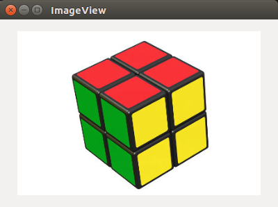
After segmentation and coloring the larger segments (except background):
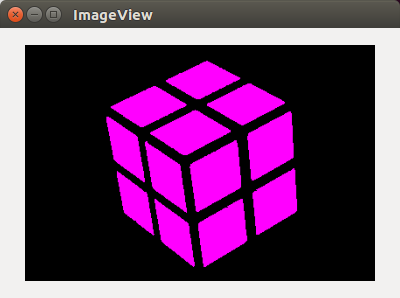
 segmented

Benchmark results:

julia> summary(img)
"270×400 Array{RGB{N0f8},2}"

julia> @benchmark fast_scanning(img, 0.21)
BenchmarkTools.Trial: 
  memory estimate:  1.94 MiB
  allocs estimate:  5636
  --------------
  minimum time:     20.537 ms (0.00% GC)
  median time:      21.222 ms (0.00% GC)
  mean time:        21.887 ms (0.60% GC)
  maximum time:     40.295 ms (0.00% GC)
  --------------
  samples:          229
  evals/sample:     1
codecov[bot] commented 7 years ago

Codecov Report

Merging #5 into master will not change coverage. The diff coverage is 100%.

Impacted file tree graph

@@          Coverage Diff          @@
##           master     #5   +/-   ##
=====================================
  Coverage     100%   100%           
=====================================
  Files           3      5    +2     
  Lines         210    281   +71     
=====================================
+ Hits          210    281   +71
Impacted Files Coverage Δ
src/core.jl 100% <ø> (ø) :arrow_up:
src/region_growing.jl 100% <100%> (ø) :arrow_up:
src/ImageSegmentation.jl 100% <100%> (ø)
src/fast_scanning.jl 100% <100%> (ø)

Continue to review full report at Codecov.

Legend - Click here to learn more Δ = absolute <relative> (impact), ø = not affected, ? = missing data Powered by Codecov. Last update 0d8720a...22e05e5. Read the comment docs.

annimesh2809 commented 7 years ago

After some more changes, the performance has increased with a mean time of about 40 ms for a 512x512 color image. However, when I tried to unify the two implementations, the performance decreased for 2-d images. Multiple data structures that are required for N-d images are not necessary for the 2-d case. Another concern is regarding the API of the functions. The methods for fast_scanning have two arguments diff_fn and threshold. These arguments could be replaced with a single argument belongs_to::Function which would return true if the pixel could belong to the region or else it would return false. Internally it could work as belongs_to(region, point) = diff_fn(region, point) < threshold. This would also allow removing the sqrt from default_diff_fn which is slowing the implementation. So it would look like:

default_diff_fn{CT1<:Colorant, CT2<:Colorant}(c1::CT1,c2::CT2) = sum(abs2,(c1)-Images.accum(CT2)(c2))
belongs_to(region, point) = default_diff_fn(region, point) < threshold^2
timholy commented 7 years ago

If unifying them is too painful, then by all means keep them separate. I am trying to head out for a holiday, but I'll see if I can review changes over the weekend. Sorry for the delay, I have been very busy with julia 1.0 changes lately...

timholy commented 7 years ago

Seems that if a couple of comments above are addressed (spell out bfs and generalize to use Real as well as Colorant) then this is good to go.

annimesh2809 commented 7 years ago

Yes, currently I am working on replacing the bfs! function with a union-find data structure to increase performance and also trying to merge the two implementations. I will try to complete this implementation with the tests and docstring by tomorrow.

annimesh2809 commented 7 years ago

After removing the bfs_color! function, it was easy to merge the two implementations without any performance loss. Now it uses a Union-find data structure to guarantee a linear time complexity on the number of pixels.

annimesh2809 commented 7 years ago
  1. The paper demonstrates that adaptive thresholding produces better segmentation with grayscale images. This can be implemented as another method for CT<:Gray using dispatch. Should we add this method?
  2. A utility function that removes the segments with pixel count < threshold might be useful. I tried searching for it but could not find what I wanted (my googling skills seem to be poor). @timholy and @tejus-gupta, have you guys worked on or know about any such algorithm? The function would assign the pixels of the smaller segments to its nearest valid segment (with pixel count > threshold).
tejus-gupta commented 7 years ago

The author's implementation of the "Efficient Graph-Based Image Segmentation" paper post processes the image to remove small segments. They construct a Region Adjacency Graph with each of the segmented region as vertex and edges between neighboring regions measuring dissimilarity between these regions. They iterate through edges (sorted in increasing order of weight) and merge an edge's two vertices if either of the vertex regions has size < minimum region size. Since edge weights measure similarity between vertex regions, small regions will merge with their most similar neighbor (and this merged region will recursively merge with it's most similar region if it's size < minimum region size).

Due to the way felzenszwalb's algorithm and normalized graph-cut algorithm are setup, their is no overhead for constructing the RAG and managing edge links during merge step. This step may slow down your algorithm. Choosing the similarity metric for the RAG that always works is also difficult.

annimesh2809 commented 7 years ago

The utility function is not specifically meant for this algorithm. It could be present in core.jl and have a prototype like:

function segfilter{T<:AbstractArray,U<:Union{Colorant, Real}}(seg::SegmentedImage{T,U}, threshold::Int)::SegmentedImage{T,U}

Provided a reasonable threshold, the fast scanning algorithm produces large enough segments. seg5

This function is just in case the user wants to set a lower limit on the size of segments, he can use any of the segmentation methods depending on his requirements and then filter it using this method.

timholy commented 7 years ago

:100: for having succeeded in merging the two implementations with no loss in performance. You're leveraging what I think is Julia's main asset, the ability to write incredibly generic code without sacrificing speed. I think it's what sets Julia apart from anything I've ever used before, and you're becoming a master at exploiting this.

I don't see anything that should hold this up from merging, unless you want to tackle the items in https://github.com/JuliaImages/ImageSegmentation.jl/pull/5#issuecomment-312744375. Would the adaptive threshold produce a different value for each pixel? If so, could you once again stick with a single implementation, allowing an AbstractArray input for thresh and then defining something like this?

getscalar(A::AbstractArray, i) = A[i]
getscalar(a::Real, i) = a

As far as merging small components goes, one possibility would be to have a function that constructs a graph from a SegmentedImage keeping track of how many times each component is adjacent to each other component. This graph will be smaller than any pixelwise graph (since it only has as many nodes as there are labels, rather than pixels) and might allow quite a few different types of post-processing.

annimesh2809 commented 7 years ago

I like the idea of allowing an AbstractArray input for thresh and using getscalar. I will add adaptive thresholding by today, then we can merge. I will add the function to merge smaller components in a separate PR.

annimesh2809 commented 7 years ago

Support for adaptive thresholding has been added. An array can be passed as threshold which partitions the original image into blocks and each block is assigned a common threshold. For grayscale images, the adpative_thres function returns the N-dimensional threshold array, given the number of partitions in each dimension. The adaptive_thres function calculates the thresholds based on the frequency(sharpness) and variance of each block. The constants have been adjusted to work with common grayscale images, however, they are dependent on the domain of the image. This does not constrain us as the user can provide custom thresholds in the form of arrays.

timholy commented 7 years ago

:fireworks: