precision of CWT

[grlee77]

I was looking at the internals of CWT to understand why it takes the integral of the wavelet here:

https://github.com/PyWavelets/pywt/blob/20f67abac3364f87dfa0136338a27444f121597d/pywt/_cwt.py#L125-L126

while SciPy's implementation does not. This appears to be because the PyWavelets implementation is doing things the way Matlab's original cwt function was implemented. Specifically it is following the algorithm listed in this old version of their toolbox documentation (The algorithm does not appear to be listed in the current version of Matlab's online documentation).

Here is a concrete example comparing to scipy.signal.cwt with the morlet2 wavelet from scipy/scipy#7076 to illustrate the issue:

import numpy as np
import matplotlib.pyplot as plt
import pywt

time, sst = pywt.data.nino()
dt = time[1] - time[0]

# Taken from http://nicolasfauchereau.github.io/climatecode/posts/wavelet-analysis-in-python/
fb = 2.0
fc = 1.0
wavelet = pywt.ContinuousWavelet('cmor{}-{}'.format(fb, fc))
scales = np.arange(1, 64)

[cfs, frequencies] = pywt.cwt(sst, scales, wavelet, dt)
power = (abs(cfs)) ** 2

from functools import partial
wav = partial(morlet2, w=2*np.pi * wavelet.center_frequency)
cfs_scipy = cwt(sst, wav, widths=scales, dtype=np.complex128)
fig, axes = plt.subplots(2, 1)
axes[0].imshow(np.abs(cfs))
axes[1].imshow(np.abs(cfs_scipy))

This gives the following results: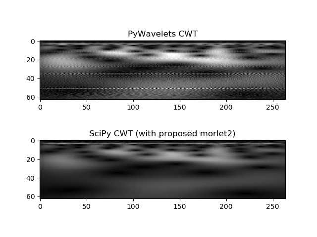

Note that there is quite a bit of zipper-like artifact in the pywt.cwt output. It seems that increasing the precision argument in the call to intwave resolves the issue. I think the value of 10 highlighted above was chosen to match Matlab, but I think we should probably switch to a larger value. For most signals, the call to intwave is probably substantially shorter than the convolution itself, so I think it should not be problematic from a computation time standpoint to increase it a bit. (The length of int_psi will be 2**precision, but this will not change the eventual downsampled int_psi_scale signal that is used during the convolutions.

The reason the zipper-like artifact occurs seems to be because this int_psi waveform is computed once, but then integer indices are used to get versions at different scales:

https://github.com/PyWavelets/pywt/blob/20f67abac3364f87dfa0136338a27444f121597d/pywt/_cwt.py#L149-L154

The actual indices corresponding to the scales would actually be floating point, not int, so rounding them to integers gives a non-uniform step size across int_psi when computing int_psi_scale. The more int_psi is oversampled, the less this is an issue.

Increasing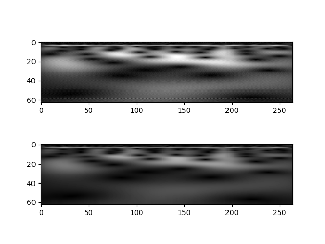 precision from 10 to 12 reduces the artifact:

and further increasing to 14 makes it no longer visible:

A separate issue from the artifact is the normalization convention used In the figures above, the overall pattern looks the same, but there is some intensity difference across scales. I think this may be due to a different convention used for normalization of the wavelets. PyWavelets (and Matlab) use a normalization constant chosen to give unit L1 norm of the wavelet, while SciPy and some textbook/literature definitions use unit L2 norm. Matlab explains the rationale for their choice here. So, I wouldn't say either toolbox is "wrong", it just seems to be a matter of the convention used. We should probably make this a bit more explicit in the docs, though.

[rgommers]

Nice detective work! Argument for changing the default value seems convincing to me.

[OverLordGoldDragon]

@grlee77 Thank you for the 'detective work', it was essential to understanding the implementation.

I've written a thorough breakdown of the implementation in three parts: (1) general; (2) resampling vs recomputing wavelet; (3) normalization. In (3), I found that the coefficients are actually L2-normalized, even though the wavelet is initially L1-normalized, and that L1 norm seems preferable. Further, the precision problem is described in detail, and I fully support your call to increase it.

I'll dig into ssqueezepy's CWT next, and also Scipy's, will be clear from there how to proceed, but if I am to go with pywt, a higher precision is a must.

[karn1986]

@grlee77 Thanks for this comment. I came across this after I opened a similar issue #705 .

The MATLAB algorithm you referenced above seems to involve two convolutions with the intwave function - one with int_psi(k+1) and another with int_psi(k) followed by elementwise differencing of the two arrays. The cwt implementation in pywt just does one convolution with int_psi(k) followed by a finite difference which results in finite differencing the adjacent coefficients. This feels incorrect. I believe it should be simply replaced by psi(k) i.e. the discretized wavelet function as proposed in #574

Here's an example of cwt computed using the current implemention for a synthetic signal

import pywt
import numpy as np
import matplotlib.pyplot as plt

t = np.linspace(0, 10, 2000, endpoint=False) # sampling frequency of 200 Hz
signal = (
        np.cos(2 * np.pi * 7 * t) + # contant 7 Hz wave
        np.real(np.exp(-7*(t-7)**2)*np.exp(1j*2*np.pi*2*(t-7))) +  # 2 Hz wave localized around t = 7
        4*np.real(np.exp(1j*2*np.pi*16*t)) * (t>7)*(t<9) + # 16 Hz between t = 7 and 9
        2*np.real(np.exp(1j*2*np.pi*32*t)) * (t>2.5)*(t<4) + # 32 Hz between t = 2.4 and 4
        8*np.real(np.exp(-((t-5)**2)/1.5)*np.exp(1j*2*np.pi*64*(t-5)))/np.sqrt(1.5*np.pi) # 64 Hz localized around t = 5
        )
scales = np.arange(2, 128)
dt = t[1] - t[0]
[coefficients, frequencies] = pywt.cwt(signal, scales, 'cmor2.0-1.0', dt)
power = (np.abs(coefficients)) ** 2
levels = [0.0625, 0.125, 0.25, 0.5, 1, 2, 4, 8]
contourlevels = np.log2(levels)

fig, ax = plt.subplots(figsize=(15, 10))
im = ax.contourf(t, np.log2(frequencies), np.log2(power), contourlevels, extend='both',cmap=plt.cm.seismic)
ax.set_ylabel('Frequency (Hz)', fontsize=18)
ax.set_xlabel('Time (sec)', fontsize=18)

yticks = 2**np.linspace(np.ceil(np.log2(frequencies.min())), np.ceil(np.log2(frequencies.max())), 10)
ax.set_yticks(np.log2(yticks))
ax.set_yticklabels(yticks)

cbar_ax = fig.add_axes([0.95, 0.5, 0.03, 0.25])
fig.colorbar(im, cax=cbar_ax, orientation="vertical")

you can clearly see lot of artifacts especially at lower frequencies. Using the solution proposed in #574 we get the following