Plug - Post on Neural ODEs

[Emmanuel-R8]

This is a shameless plug for a post on Normalising flows and Neural ODEs. Short on Julia code for the moment but this is in the works.

I wanted to make any parts of the post available to be pilfered if anything can be used in the documentation. Otherwise comments welcome.

https://emmanuel-r8.github.io/post/2020/09/11/normalising-flows/

[ChrisRackauckas]

Thanks for sharing. Let us know if you need any help putting together the Julia version.

[Emmanuel-R8]

Calling on the offer.

The post includes an example which basically replicates a multimodal 2D distribution from a PyTorch library. See [https://torchdyn.readthedocs.io/en/latest/tutorials/07a_continuous_normalizing_flows.html]().

The following is an attempt at a Julia translation using FFJORD. Despite my best efforts, it bombs out at the end of the attached code before finishing a single iteration. All the same whether using 1 or 2 dimensions. . Julia = 1.5.2, DiffEqFlux = 1.24, Flux = 0.11.1

Any advice?

using Random, Distributions, Plots, LinearAlgebra

n_samples = 1 << 9
n_gaussians = 6
n_dims = 2

# Translated from Torchdyn ToyDataset()

# :param n_samples::int : number of data points in the generated dataset
# :param n_gaussians::int : number of gaussians distributions placed on the circle of radius `radius`
# :param radius:: int : radius of the circle on which the distributions lie
#  :param std_gaussians::int : standard deviation of the gaussians.
#  :param noise:: float32 : standard deviation of noise magnitude added to each data point
function generate_gaussians(; n_dims = n_dims, n_samples=100, n_gaussians=7, 
        radius=1.f0, std_gaussians=0.2f0, noise=0.001f0)

    x = zeros(Float32, n_dims, n_samples * n_gaussians)
    y = zeros(Float32, n_samples * n_gaussians)
    incremental_angle = 2 * π / n_gaussians

    dist_gaussian = MvNormal(n_dims, sqrt(std_gaussians))

    if n_dims > 2
        dist_noise = MvNormal(n_dims - 2, sqrt(noise))
    end

    current_angle = 0.f0
    for i ∈ 1:n_gaussians
        current_loc = zeros(Float32, n_dims, 1)
        if n_dims >= 1
            current_loc[1] = radius * cos(current_angle)
        end

        if n_dims >= 2
            current_loc[2] = radius * sin(current_angle)
        end

        x[1:n_dims, (i-1)*n_samples+1:i*n_samples] = current_loc[1:n_dims] .+ rand(dist_gaussian, n_samples)
        if n_dims > 2
            x[1:n_dims-2, (i-1)*n_samples+1:i*n_samples] = rand(noise, n_samples)
        end

        y[   (i-1)*n_samples+1:i*n_samples] = Float32(i) .* ones(Float32, n_samples)

        current_angle = current_angle + incremental_angle
    end

    return x, y
end

X, Y = generate_gaussians(; n_samples = n_samples ÷ n_gaussians, 
                            n_gaussians = n_gaussians, 
                            radius = 4.0f0, 
                            std_gaussians = 0.5f0)
X = (X .- mean(X)) ./ std(X)
X_SIZE = size(X)[2]

# We will continue onward using the GR backend
gr() 
if n_dims == 1
    histogram(X[1, :], title = "Sample from the true density")
else
    scatter(X[1, :], X[2, :], title = "Sample from the true density", markershape=:x, markersize=2)
end

using DiffEqFlux, Optim, OrdinaryDiffEq, Zygote, Flux

f = Chain(Dense(n_dims, 16 * n_dims, tanh), 
          Dense(16 * n_dims, 16 * n_dims, tanh), 
          Dense(16 * n_dims, 16 * n_dims, tanh), 
          Dense(16 * n_dims, n_dims, tanh))

t_span = (0., 1.)
cnf_ffjord = FFJORD(f, t_span, Tsit5(), basedist = MvNormal(n_dims, 1.), monte_carlo = true)

function loss_adjoint_orig(θ)
    logpx = cnf_ffjord(X, θ)[1]
    return -mean(logpx)[1]
end

# callback function to observe training
cb = function()
    global iter += 1
    println("Iteration $iter")
end

# Train using the ADAM optimizer
iter = 0
res1 = DiffEqFlux.sciml_train(
        loss_adjoint_orig, 
        cnf_ffjord.p,
        ADAM(0.1), 
        cb = cb,
        maxiters = 10)

    MethodError: no method matching (::var"#11#12")(::Array{Float32,1}, ::Float32)

    Stacktrace:
     [1] macro expansion at /home/emmanuel/.julia/packages/DiffEqFlux/8UHw5/src/train.jl:123 [inlined]
     [2] macro expansion at /home/emmanuel/.julia/packages/ProgressLogging/BBN0b/src/ProgressLogging.jl:328 [inlined]
     [3] (::DiffEqFlux.var"#73#78"{var"#11#12",Int64,Bool,Bool,typeof(loss_adjoint_orig),Array{Float32,1},Params})() at /home/emmanuel/.julia/packages/DiffEqFlux/8UHw5/src/train.jl:64
     [4] with_logstate(::Function, ::Any) at ./logging.jl:408
     [5] with_logger at ./logging.jl:514 [inlined]
     [6] maybe_with_logger(::DiffEqFlux.var"#73#78"{var"#11#12",Int64,Bool,Bool,typeof(loss_adjoint_orig),Array{Float32,1},Params}, ::LoggingExtras.TeeLogger{Tuple{LoggingExtras.EarlyFilteredLogger{ConsoleProgressMonitor.ProgressLogger,DiffEqFlux.var"#68#70"},LoggingExtras.EarlyFilteredLogger{Base.CoreLogging.SimpleLogger,DiffEqFlux.var"#69#71"}}}) at /home/emmanuel/.julia/packages/DiffEqFlux/8UHw5/src/train.jl:39
     [7] sciml_train(::Function, ::Array{Float32,1}, ::ADAM, ::Base.Iterators.Cycle{Tuple{DiffEqFlux.NullData}}; cb::Function, maxiters::Int64, progress::Bool, save_best::Bool) at /home/emmanuel/.julia/packages/DiffEqFlux/8UHw5/src/train.jl:63
     [8] top-level scope at In[124]:3
     [9] include_string(::Function, ::Module, ::String, ::String) at ./loading.jl:1091
     [10] execute_code(::String, ::String) at /home/emmanuel/.julia/packages/IJulia/rWZ9e/src/execute_request.jl:27
     [11] execute_request(::ZMQ.Socket, ::IJulia.Msg) at /home/emmanuel/.julia/packages/IJulia/rWZ9e/src/execute_request.jl:86
     [12] #invokelatest#1 at ./essentials.jl:710 [inlined]
     [13] invokelatest at ./essentials.jl:709 [inlined]
     [14] eventloop(::ZMQ.Socket) at /home/emmanuel/.julia/packages/IJulia/rWZ9e/src/eventloop.jl:8
     [15] (::IJulia.var"#15#18")() at ./task.jl:356

[Vaibhavdixit02]

The callback needs to allow 2 args, just make it be

cb = function(x,l)
    global iter += 1
    println("Iteration $iter")
end

and it should work

[Emmanuel-R8]

Did the trick. Thanks a lot.

I never thought about looking there to find the error since I used the Augmented NODE callback [https://diffeqflux.sciml.ai/dev/examples/augmented_neural_ode/#Callback-Function-1]() which has no parameters.

[avik-pal]

@Emmanuel-R8 the reason for that is sciml_train and Flux.train! have different requirements for the callback function. The augmented NODE example uses the latter.

[Emmanuel-R8]

Thanks Avik

I used this callback because the CNF example uses a callback ("cb=cb") which is not defined. So I went sniffing around. When I have a bit of time, I'll work on a PR to improve the docs with the benefit of this discussion.

[Emmanuel-R8]

Despite playing with the code in ffjord.jl code for a few hours, I still find myself unable to fully use the model. I have a 2D model cnf_ffjord and a set of trained parameters res1. I want to be able to do several things:

1. In the generative direction, for a given random value, generate a data point.
2. In the opposite encoding direction, for a given data point, flow back to the simple multinormal distribution.
3. As a corollary of 2, given a data point, get its probability. I use cnf_ffjord([x, y], res1.minimizer; monte_carlo=false) to do that. Running that over a range of values gives a min of -9 and max of 29. Clearly I don't pass the right parameters or I don' t understand what cnf_ffjord does.

[ChrisRackauckas]

@DhairyaLGandhi could we get some help here?

[Emmanuel-R8]

@DhairyaLGandhi

Anything I can provide to assist?

[ChrisRackauckas]

Oh actually it's probably @d-netto that would be able to comment on that function, sorry.

[DhairyaLGandhi]

You'd also have to return a bool from the callback as sciml_train expects. I was able to train the model by eliminating the callback, since it isn't doing anything at the moment. One other quick change I made was

f = Chain(Dense(n_dims, 16 * n_dims, tanh), 
          Dense(16 * n_dims, 16 * n_dims, tanh), 
          Dense(16 * n_dims, 16 * n_dims, tanh), 
          Dense(16 * n_dims, n_dims, tanh)) |> Flux.f64    # <- note this

[Emmanuel-R8]

The issue is convergence (I'll ignore speed for the moment). By plotting intermediate steps, I discovered it is an absolute dog's breakfast.

I am trying to learn 6 normal distributions located on an hexagon:

Here are 2 series of plots each showing about 20 learning steps using ADAM. The former is with ADAM(0.1). The latter is with ADAM(0.02)

I now understand why trying to understand the training results was a road to nowhere. In the former, the plot is lost within 2 iterations. In the latter, it is a bit better but still not able to learn 6 modes, unlike the Torchdyn library (plot from my post):

.

Any advice on how to improve convergence (get any at all)?

[ChrisRackauckas]

@d-netto let's talk about this.

[avik-pal]

# Code for Sampling
pz = cnf_ffjord.basedist
Z_samples = rand(pz, 512) |> gpu
sense = InterpolatingAdjoint()
ffjord_ = (u, p, t) -> DiffEqFlux.ffjord(u, p, t, cnf_ffjord.re, e, false, false)
e = cu(randn(eltype(X), size(Z_samples)))
_z = Zygote.@ignore similar(X, 1, size(Z_samples, 2))
Zygote.@ignore fill!(_z, 0.0f0)
prob = ODEProblem{false}(ffjord_, vcat(Z_samples, _z), (1.0, 0.0), res1.minimizer)
x_gen = solve(prob, cnf_ffjord.args...; sensealg = sense, cnf_ffjord.kwargs...)[1:end-1, :, end]
scatter(x_gen[1, :], x_gen[2, :], title = "Testing", markershape=:x, markersize=2)

@Emmanuel-R8 There are a couple of suggestions I would make:

• Train with a learning rate of ~ 0.001 (torchdyn code uses 2e-3)
• There is no need for the activation function after the last layer
• 10 iterations is very little. The results I posted are after 100 iterations.
• As for the performance, doing a backprop with a batch size of 512 is expected to be very slow on CPU. On GPU the training for 100 iterations takes only 1.38 mins on my local setup.

A good starting point is to always use the hyperparameters (+ model architecture) from a code that is known to work.

[avik-pal]

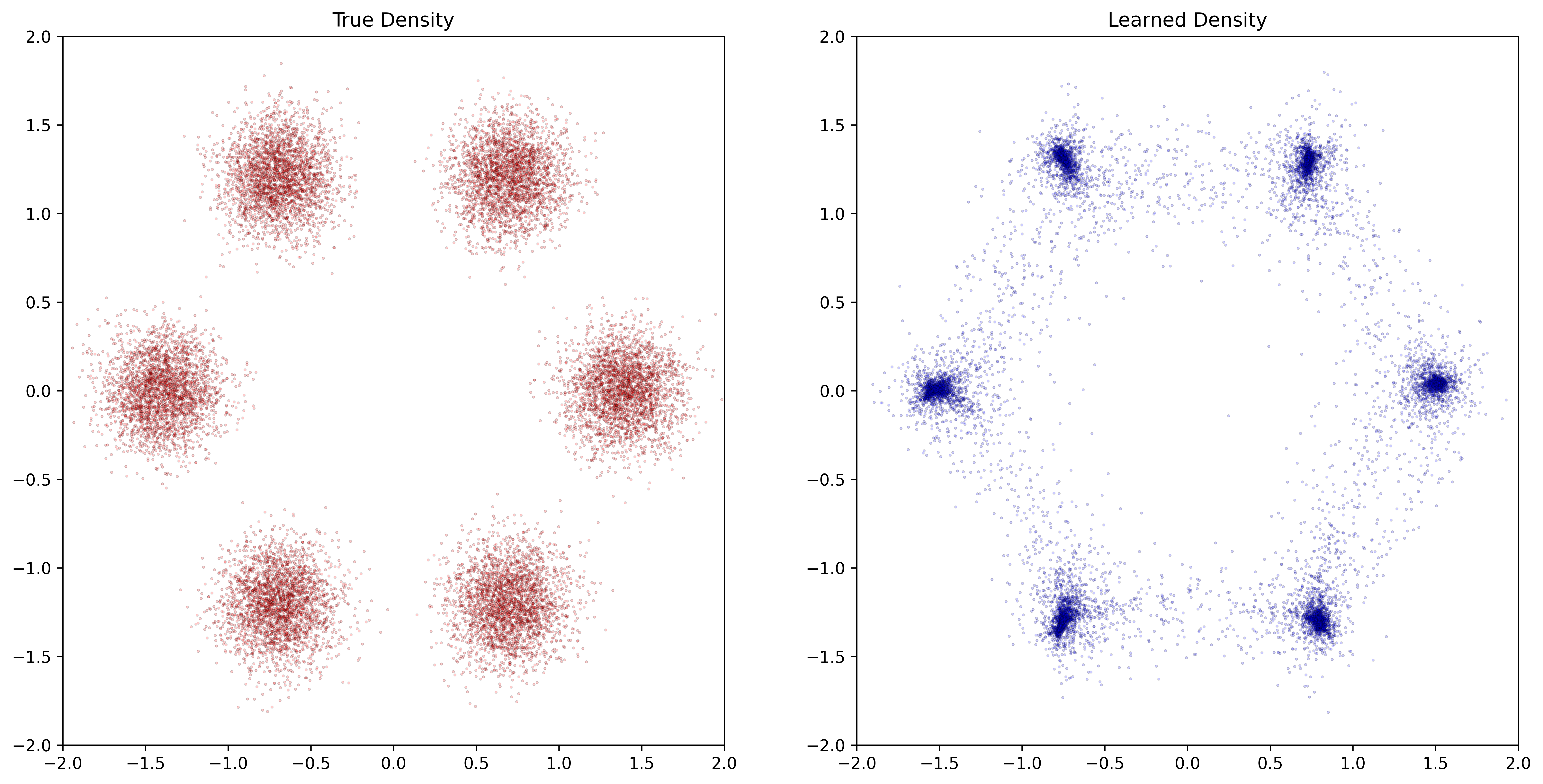
The previous plot was of something else. This is the correct version.

[Emmanuel-R8]

Thanks.

I don' t have a GPU, and I haven' t yet succeeded to make Colab comply with my wishes. I'll need a few hours to check on my side.

[Emmanuel-R8]

My laptop is still churning along.

I am sharing where I am at on a Colab notebook. Not asking for review, but it took me a while to get that working, so I assume it will be useful to some.

https://colab.research.google.com/drive/1xbeWxgwrToZBYg8KxUOPjraoLrHrXbEJ?usp=sharing

[Emmanuel-R8]

Wrong link. This is the one:

https://colab.research.google.com/drive/15mBDXEfEv7Yg1t9Euw7CMFvKyQyNdh1f?usp=sharing

[Emmanuel-R8]

That's 100 iterations with 2e-3. A lot better. Thanks for the guidance.