 baggepinnen
commented
2 years ago
baggepinnen
commented
2 years ago Hi @LiborKudela !
Are you solving to the same tolerances with both MTK and modelica?
Closed LiborKudela closed 1 month ago
baggepinnen
commented
2 years ago Hi @LiborKudela !
Are you solving to the same tolerances with both MTK and modelica?
 ChrisRackauckas
commented
2 years ago
ChrisRackauckas
commented
2 years ago  LiborKudela
commented
2 years ago
LiborKudela
commented
2 years ago Sorry for the delay.. A lot of compilation time with some of these variants.. I had to terminate many I think they would not come to an end
Are you solving to the same tolerances with both MTK and modelica?
Yes, both are set to 1e-6. As well as the saveat=100 equivalent in OMC.
- autodiff=false shouldn't matter if jac=true?
when autodiff=true first call to solve takes much longer time (for higher N) otherwise no effect -> that might be a bug
- is sparse truly better here?
Well, the derivations of the states need only few other states around it so it should be better, but I will check.
- Did you try FBDF? That's close to CVODE/IDA
sparse= false -> no effect, which I actually did not expect

- How does CVODE do? Or IDA from Julia?
sparse=true, I could not make any DAE form solve faster inluding IDA. I have got a lot of crashes with dae form.
I might not be using the IDA correctly.
the CVODE_BDF works and also scales bad.

- Which linear solver? Did you try KLU?
I did try KLU but it gave me an Error so I moved on. Now when I se the Error again I have questions.
solve(prob, QNDF(autodiff=false, linsolve = KLUFactorization()), reltol=1e-6, abstol=1e-6, saveat=100)
ERROR: MethodError: no method matching KLU.KLUFactorization(::Matrix{Float64})Which is weird because i have set sparse=true in ODAEProblem so why it passes in non sparse matrix?
Btw I also get this warnings comming from solve
Unrecognized keyword arguments: [:jac, :sparse]Is it posible that the sparsity matrix and jacobian are not comming through from prob or something? How can we check that?
ChrisRackauckas
commented
2 years ago Share ]st.
LiborKudela
commented
2 years ago [6e4b80f9] BenchmarkTools v1.3.1 [336ed68f] CSV v0.10.4 [052768ef] CUDA v3.11.0 [a93c6f00] DataFrames v1.3.4 [82cc6244] DataInterpolations v3.9.2 [39dd38d3] Dierckx v0.5.2 [aae7a2af] DiffEqFlux v1.51.2 [41bf760c] DiffEqSensitivity v6.79.0 [0c46a032] DifferentialEquations v7.2.0 [f6369f11] ForwardDiff v0.10.30 [615f187c] IfElse v0.1.1 [a98d9a8b] Interpolations v0.14.0 [ef3ab10e] KLU v0.3.0 [7f56f5a3] LSODA v0.7.0 [b964fa9f] LaTeXStrings v1.3.0 [7ed4a6bd] LinearSolve v1.20.0 [eff96d63] Measurements v2.7.2 [961ee093] ModelingToolkit v8.15.1 [7f7a1694] Optimization v3.7.1 [1dea7af3] OrdinaryDiffEq v6.18.1 [f0f68f2c] PlotlyJS v0.18.8 [91a5bcdd] Plots v1.31.2 [f27b6e38] Polynomials v3.1.4 [1fd47b50] QuadGK v2.4.2 [731186ca] RecursiveArrayTools v2.31.1 [276daf66] SpecialFunctions v2.1.7 [43dc94dd] SteamTables v1.3.0 [c3572dad] Sundials v4.9.4 [0c5d862f] Symbolics v4.9.0 [a759f4b9] TimerOutputs v0.5.20 [95ff35a0] XSteam v0.3.0
LiborKudela
commented
2 years ago Great news!! (sort of) The problem with sparsity and KLU not working is only happening with ODAEProblem. I have tried pure ODEProblem so we have a non-singular mass matrix:
tspan = (0.0, 19*3600)
@named testbench = TestBenchPreinsulated(L=470, N=160, dn=0.3127, t_layer=[0.0056, 0.058])
sys = structural_simplify(testbench)
prob = ODEProblem(sys, [], tspan, jac=true, sparse=true)
prob.u0 .= 12
@time sol = solve(prob, QBDF(linsolve=KLUFactorization()), reltol=1e-6, abstol=1e-6, saveat=100);
@time sol = solve(prob, CVODE_BDF(linear_solver=:KLU), reltol=1e-6, abstol=1e-6, saveat=100);
Result: 😄 I knew that Julia should be faster.

But when I go from N=160 to N=320 it gets stuck at compilation and never actually runs. My computer at home has only 16GB of RAM and it gets pushed to limit. I will try it at school tomorrow on bigger machine, but this should be probably addressed? OpenModelica compiles this sizes easily even on my home PC.
ChrisRackauckas
commented
2 years ago Modelica defaults to KLU. I just did a bunch of tests and it makes sense for us too, so I changed the default linear solver. UMFPACK is rarely better.
As for the compilation time, this is a known issue with MTK that is being worked on.
 YingboMa
commented
1 year ago
YingboMa
commented
1 year ago Hey, could you run the above benchmark again using the latest MTK? It should be able to handle larger systems now.
LiborKudela
commented
1 year ago Hi, I will run it later today. Thank you!
LiborKudela
commented
1 year ago @YingboMa, I have run the benchmark.
First I have updated everything.
Julia version: 1.8.2
]st : [615f187c] IfElse v0.1.1 [7ed4a6bd] LinearSolve v1.27.0 [961ee093] ModelingToolkit v8.29.1 [1dea7af3] OrdinaryDiffEq v6.29.3 [91a5bcdd] Plots v1.35.4 [f27b6e38] Polynomials v3.2.0 [0c5d862f] Symbolics v4.13.0 [95ff35a0] XSteam v0.3.
I have also changed the symbolic arrays from A[1:N](t) to (A(t))[1:N] since the former is deprecated in Symbolics.
I have run only the ODEProblem version of the benchmark.
The test machine is a Linux machine with 16GB of RAM, the OS is Ubuntu 20.04 (freshly updated).
I am unable to run N=1280 with Tsit5() solver - it crashes the process (in VScode), because it eats all the RAM
I am unable to run N=320 with QBDF(linsolve=KLUFactorization()) solver with the same result as the above
I was able to run the OpenModelica version of the model with N=2560 on this machine relative fast (simulation time 10.5s)
Should I change something more in the script to take advantage of the new version of MTK?
The script I used for this test:
using ModelingToolkit, OrdinaryDiffEq, Symbolics, IfElse, XSteam,
      Polynomials, Plots, LinearSolve

#          o  o  o  o  o  o  o < heat capacitors
#          |  |  |  |  |  |  | < heat conductors
#          o  o  o  o  o  o  o
#          |  |  |  |  |  |  |
#Source -> o--o--o--o--o--o--o -> Sink
#       advection diff source PDE

@variables t
D = Differential(t)
m_flow_source(t) = 2.75
T_source(t) = (t>12*3600)*56.0 + 12.0
@register_symbolic m_flow_source(t)
@register_symbolic T_source(t)

#build polynomial liquid-water property only dependent on Temperature
p_l = 5 #bar
T_vec = collect(1:1:150);
kin_visc_T = fit(T_vec, my_pT.(p_l, T_vec)./rho_pT.(p_l, T_vec), 5);
lambda_T = fit(T_vec, tc_pT.(p_l, T_vec), 3);
Pr_T = fit(T_vec, 1e3*Cp_pT.(p_l, T_vec).*my_pT.(p_l, T_vec)./tc_pT.(p_l, T_vec), 5);
rho_T = fit(T_vec, rho_pT.(p_l, T_vec), 4);
rhocp_T = fit(T_vec, 1000*rho_pT.(p_l, T_vec).*Cp_pT.(p_l, T_vec), 5);

@connector function FluidPort(;name, p=101325.0, m=0.0, T=0.0)
    sts = @variables p(t)=p m(t)=m [connect=Flow] T(t)=T [connect=Stream]
    ODESystem(Equation[], t, sts, []; name=name)
end

@connector function VectorHeatPort(;name, N=100, T0=0.0, Q0=0.0)
    #TODO: Vector of flow vars warning but eqs are correct!!
    sts = @variables (T(t))[1:N]=T0 (Q(t))[1:N]=Q0 [connect=Flow]
    ODESystem(Equation[], t, [T; Q], []; name=name)
end

#Taylor-aris dispersion model
function Dxx_coeff(u, d, T)
    Re = abs(u)*d/kin_visc_T(T) + 0.1
    IfElse.ifelse(Re < 1000, (d^2/4)*u^2/48/0.14e-6, d*u*(1.17e9*Re^(-2.5) + 0.41))
end

#Nusselt number model
function Nusselt(Re, Pr, f)
    IfElse.ifelse(Re <= 2300, 3.66,
    IfElse.ifelse(Re <= 3100, 3.5239*(Re/1000)^4-45.158*(Re/1000)^3+212.13*(Re/1000)^2-427.45*(Re/1000)+316.08,
                  f/8*((Re-1000)*Pr)/(1+12.7*(f/8)^(1/2)*(Pr^(2/3)-1))))
end

#Darcy weisbach friction factor
function Churchill_f(Re, epsilon, d)
    theta_1 = (-2.457*log(((7/Re)^0.9)+(0.27*(epsilon/d))))^16
    theta_2 = (37530/Re)^16
    8*((((8/Re)^12)+(1/((theta_1+theta_2)^1.5)))^(1/12))
end

function FluidRegion(;name, L=1.0, dn=0.05, N=100, T0=0.0,
                     lumped_T=50, diffusion=true, e=1e-4)
    @named inlet = FluidPort()
    @named outlet = FluidPort()
    @named heatport = VectorHeatPort(N=N)

    dx=L/N
    c=[-1/8, -3/8, -3/8] # advection stencil coeficients
    A = pi*dn^2/4

    p = @parameters C_shift = 0.0 Rw = 0.0 # stuff for latter
    @variables begin
        (T(t))[1:N] = fill(T0, N)
        Twall(t)[1:N] = fill(T0, N)
        (S(t))[1:N] = fill(T0, N)
        (C(t))[1:N] = fill(1.0, N)
        u(t) = 1e-6
        Re(t) = 1000.0
        Dxx(t) = 0.0
        Pr(t) = 1.0
        alpha(t) = 1.0
        f(t) = 1.0
    end

    sts = [T..., Twall..., S..., C..., u, Re, Dxx, Pr, alpha, f]

    eqs = [
        Re ~ 0.1 + dn*abs(u)/kin_visc_T(lumped_T)
        Pr ~ Pr_T(lumped_T)
        f ~ Churchill_f(Re, e, dn) #Darcy-weisbach
        alpha ~ Nusselt(Re, Pr, f)*lambda_T(lumped_T)/dn
        Dxx ~ diffusion*Dxx_coeff(u, dn, lumped_T)
        inlet.m ~ -outlet.m
        inlet.p ~ outlet.p
        inlet.T ~ instream(inlet.T)
        outlet.T ~ T[N]
        u ~ inlet.m/rho_T(inlet.T)/A
        [C[i] ~ dx*A*rhocp_T(T[i]) for i in 1:N]
        [S[i] ~ heatport.Q[i] for i in 1:N]
        [Twall[i] ~ heatport.T[i] for i in 1:N]

        #source term
        [S[i] ~ (1/(1/(alpha*dn*pi*dx)+abs(Rw/1000)))*(Twall[i] - T[i]) for i in 1:N]

        #second order upwind + diffusion + source
        D(T[1]) ~ u/dx*(inlet.T - T[1]) + Dxx*(T[2]-T[1])/dx^2 + S[1]/(C[1]-C_shift)
        D(T[2]) ~ u/dx*(c[1]*inlet.T - sum(c)*T[1] + c[2]*T[2] + c[3]*T[3]) + Dxx*(T[1]-2*T[2]+T[3])/dx^2 + S[2]/(C[2]-C_shift)
        [D(T[i]) ~ u/dx*(c[1]*T[i-2] - sum(c)*T[i-1] + c[2]*T[i] + c[3]*T[i+1]) + Dxx*(T[i-1]-2*T[i]+T[i+1])/dx^2 + S[i]/(C[i]-C_shift) for i in 3:N-1]
        D(T[N]) ~ u/dx*(T[N-1] - T[N]) + Dxx*(T[N-1]-T[N])/dx^2 + S[N]/(C[N]-C_shift)
    ]

    ODESystem(eqs, t, sts, p; systems=[inlet, outlet, heatport], name=name)
end

function Cn_circular_wall_inner(d, D, cp, ρ)
    C = pi/4*(D^2-d^2)*cp*ρ
    return C/2
end

function Cn_circular_wall_outer(d, D, cp, ρ)
    C = pi/4*(D^2-d^2)*cp*ρ
    return C/2
end

function Ke_circular_wall(d, D, λ)
    2*pi*λ/log(D/d)
end

function CircularWallFEM(;name, L=100, N=10, d=0.05, t_layer=[0.002],
                         λ=[50], cp=[500], ρ=[7850], T0=0.0)
    @named inner_heatport = VectorHeatPort(N=N)
    @named outer_heatport = VectorHeatPort(N=N)
    dx = L/N
    Ne = length(t_layer)
    Nn = Ne + 1
    dn = vcat(d, d .+ 2.0.*cumsum(t_layer))
    Cn = zeros(Nn)
    Cn[1:Ne] += Cn_circular_wall_inner.(dn[1:Ne], dn[2:Nn], cp, ρ).*dx
    Cn[2:Nn] += Cn_circular_wall_outer.(dn[1:Ne], dn[2:Nn], cp, ρ).*dx
    p = @parameters C_shift=0.0
    Ke = Ke_circular_wall.(dn[1:Ne], dn[2:Nn], λ).*dx
    @variables begin
        (Tn(t))[1:N, 1:Nn] = fill(T0, N, Nn)
        (Qe(t))[1:N, 1:Ne] = fill(T0, N, Ne)
    end
    sts = [vec(Tn); vec(Qe)]
    eqs = [
        [inner_heatport.T[i] ~ Tn[i,1] for i in 1:N]
        [outer_heatport.T[i] ~ Tn[i,Nn] for i in 1:N]
        [Qe[i,j] ~ Ke[j]*(-Tn[i,j+1]+Tn[i,j]) for i in 1:N for j in 1:Ne]...
        [D(Tn[i,1])*(Cn[1]+C_shift) ~ inner_heatport.Q[i]-Qe[i,1] for i in 1:N]
        [D(Tn[i,j])*Cn[j] ~ Qe[i,j-1]-Qe[i,j] for i in 1:N for j in 2:Nn-1]...
        [D(Tn[i,Nn])*Cn[Nn] ~ Qe[i,Ne]+outer_heatport.Q[i] for i in 1:N]
    ]
    ODESystem(eqs, t, sts, p; systems=[inner_heatport, outer_heatport], name=name)
end

function CylindricalSurfaceConvection(;name, L=100, N=100, d=1.0, α=5.0)
    dx = L/N
    S = pi*d*dx
    @named heatport = VectorHeatPort(N=N)
    sts = @variables Tenv(t)=0.0
    eqs = [
        Tenv ~ 18.0
        [heatport.Q[i] ~ α*S*(heatport.T[i]-Tenv) for i in 1:N]
    ]

    ODESystem(eqs, t, sts, []; systems=[heatport], name=name)
end

function PreinsulatedPipe(;name, L=100.0, N=100.0, dn=0.05, T0=0.0, t_layer=[0.004, 0.013],
    λ=[50, 0.04], cp=[500, 1200], ρ=[7800, 40], α=5.0,
    e=1e-4, lumped_T=50, diffusion=true)
    @named inlet = FluidPort()
    @named outlet = FluidPort()
    @named fluid_region = FluidRegion(L=L, N=N, dn=dn, e=e, lumped_T=lumped_T, diffusion=diffusion)
    @named shell = CircularWallFEM(L=L, N=N, d=dn, t_layer=t_layer, λ=λ, cp=cp, ρ=ρ)
    @named surfconv = CylindricalSurfaceConvection(L=L, N=N, d=dn+2.0*sum(t_layer), α=α)
    systems = [fluid_region, shell, inlet, outlet, surfconv]
    eqs = [
        connect(fluid_region.inlet, inlet)
        connect(fluid_region.outlet, outlet)
        connect(fluid_region.heatport, shell.inner_heatport)
        connect(shell.outer_heatport, surfconv.heatport)
        ]
    ODESystem(eqs, t, [], []; systems=systems, name=name)
end

function Source(;name, p_feed=100000)
    @named outlet = FluidPort()
    sts = @variables m_flow(t)=1e-6
    eqs = [
        m_flow ~ m_flow_source(t)
        outlet.m ~ -m_flow
        outlet.p ~ p_feed
        outlet.T ~ T_source(t)
        ]
    compose(ODESystem(eqs, t, sts, []; name=name), [outlet])
end

function Sink(;name)
    @named inlet = FluidPort()
    eqs = [
        inlet.T ~ instream(inlet.T)
        ]
    compose(ODESystem(eqs, t, [], []; name=name), [inlet])
end

function TestBenchPreinsulated(;name, L=1.0, dn=0.05, t_layer=[0.0056, 0.013], N=100, diffusion=true, lumped_T=20)
    @named pipe = PreinsulatedPipe(L=L, dn=dn, N=N, diffusion=diffusion, t_layer=t_layer, lumped_T=lumped_T)
    @named source = Source()
    @named sink = Sink()
    subs = [source, pipe, sink]
    eqs = [
           connect(source.outlet, pipe.inlet)
           connect(pipe.outlet, sink.inlet)
          ]
    compose(ODESystem(eqs, t, [], []; name=name), subs)
end

function test_speed(N; solver=Tsit5())
    tspan = (0.0, 19*3600)
    @named testbench = TestBenchPreinsulated(L=470, N=N, dn=0.3127, t_layer=[0.0056, 0.058])
    sys = structural_simplify(testbench)
    prob = ODEProblem(sys, [], tspan, jac=true, sparse=true)
    prob.u0[:] .= 12.0
    #TODO: unrecognized keywords jac and sparse in solve??
    solve(prob, solver, reltol=1e-6, abstol=1e-6, saveat=100);
    return @elapsed solve(prob, solver, reltol=1e-6, abstol=1e-6, saveat=100);
end

test_speed(1280)

# scaling tests
N_x = [5, 10, 20, 40, 80, 160, 320, 640, 1280]
N_states = 4 .* N_x
OMC_IDA_470 = [0.0125157, 0.0106602, 0.0172244, 0.0255715,
               0.0567469, 0.126823, 0.247737, 0.622899, 1.32534]

JULIA_ODAE_Tsit5 = zeros(length(N_x))
for i in 1:length(N_x)
    JULIA_ODAE_Tsit5[i] = test_speed(N_x[i], solver=Tsit5())
end
println(JULIA_ODAE_Tsit5)
#[0.071787957, 0.077838405, 0.095070696, 0.136035788, 0.227302308, 0.422744682, 0.90749644, 1.906403591, NaN]

JULIA_ODAE_QNDF = zeros(length(N_x))
for i in 1:length(N_x)
    JULIA_ODAE_QNDF[i] = test_speed(N_x[i], solver=QBDF(linsolve=KLUFactorization()))
end
println(JULIA_ODAE_QNDF)

fig = plot(N_x, OMC_IDA, label="OMC IDA",
           legend=:topleft, yscale=:log10, xscale=:log10,
           xlim=(1,10000), ylim=(1e-3, 1e2), marker=:circle)
plot!(N_x, JULIA_ODAE_Tsit5, label="Julia ODAE Tsit5", marker=:square)
plot!(N_x, JULIA_ODAE_QNDF, label="Julia ODAE QNDF", marker=:star)
savefig(fig,"Scaling experiment.png")
Thanks for taking the time to run it again. For large and complex systems, symbolically computing the Jacobian won't be a good idea because the size of the expression will blowup, so I suggest you to use
prob = ODEProblem(sys, [], tspan, sparse=true)Also, we are now defaulting to KLU for sparse matrices with moderate size, so you can just use QBDF(autodiff=false), QNDF(autodiff=false), or FBDF(autodiff=false).
YingboMa
commented
1 year ago BTW, the warning is fixed in https://github.com/SciML/ModelingToolkit.jl/pull/1895
LiborKudela
commented
1 year ago Results with jac=false.
Julia run from terminal/bash (no VScode involved).

N=1280 and above still causes crashes for both the Tsit5() and QNDF(autodiff=false).
The process runs out of RAM and gets killed.
YingboMa
commented
1 year ago I have modified the script a bit to make it friendlier to the compiler. Could you try this as well?
using ModelingToolkit, OrdinaryDiffEq, Symbolics, IfElse, XSteam,
      Polynomials, Plots, LinearSolve

#          o  o  o  o  o  o  o < heat capacitors
#          |  |  |  |  |  |  | < heat conductors
#          o  o  o  o  o  o  o
#          |  |  |  |  |  |  |
#Source -> o--o--o--o--o--o--o -> Sink
#       advection diff source PDE

@variables t
D = Differential(t)
m_flow_source(t) = 2.75
T_source(t) = (t>12*3600)*56.0 + 12.0
@register_symbolic m_flow_source(t)
@register_symbolic T_source(t)

#build polynomial liquid-water property only dependent on Temperature
p_l = 5 #bar
T_vec = collect(1:1:150);
@noinline @generated kin_visc_T(t) = :(Base.evalpoly(t, $(fit(T_vec, my_pT.(p_l, T_vec)./rho_pT.(p_l, T_vec), 5).coeffs...,)))
@noinline @generated lambda_T(t)   = :(Base.evalpoly(t, $(fit(T_vec, tc_pT.(p_l, T_vec), 3).coeffs...,)))
@noinline @generated Pr_T(t)       = :(Base.evalpoly(t, $(fit(T_vec, 1e3*Cp_pT.(p_l, T_vec).*my_pT.(p_l, T_vec)./tc_pT.(p_l, T_vec), 5).coeffs...,)))
@noinline @generated rho_T(t)      = :(Base.evalpoly(t, $(fit(T_vec, rho_pT.(p_l, T_vec), 4).coeffs...,)))
@noinline @generated rhocp_T(t)    = :(Base.evalpoly(t, $(fit(T_vec, 1000*rho_pT.(p_l, T_vec).*Cp_pT.(p_l, T_vec), 5).coeffs...,)))
@register_symbolic kin_visc_T(t)
@register_symbolic lambda_T(t)
@register_symbolic Pr_T(t)
@register_symbolic rho_T(t)
@register_symbolic rhocp_T(t)

@connector function FluidPort(;name, p=101325.0, m=0.0, T=0.0)
    sts = @variables p(t)=p m(t)=m [connect=Flow] T(t)=T [connect=Stream]
    ODESystem(Equation[], t, sts, []; name=name)
end

@connector function VectorHeatPort(;name, N=100, T0=0.0, Q0=0.0)
    sts = @variables (T(t))[1:N]=T0 (Q(t))[1:N]=Q0 [connect=Flow]
    ODESystem(Equation[], t, [T; Q], []; name=name)
end

@register_symbolic Dxx_coeff(u, d, T)
#Taylor-aris dispersion model
@noinline function Dxx_coeff(u, d, T)
    Re = abs(u)*d/kin_visc_T(T) + 0.1
    IfElse.ifelse(Re < 1000, (d^2/4)*u^2/48/0.14e-6, d*u*(1.17e9*Re^(-2.5) + 0.41))
end

@register_symbolic Nusselt(Re, Pr, f)
#Nusselt number model
@noinline function Nusselt(Re, Pr, f)
    if Re <= 2300
        3.66
    elseif Re <= 3100
        3.5239*(Re/1000)^4-45.158*(Re/1000)^3+212.13*(Re/1000)^2-427.45*(Re/1000)+316.08
    else
        f/8*((Re-1000)*Pr)/(1+12.7*(f/8)^(1/2)*(Pr^(2/3)-1))
    end
end

@register_symbolic Churchill_f(Re, epsilon, d)
#Darcy weisbach friction factor
@noinline function Churchill_f(Re, epsilon, d)
    theta_1 = (-2.457*log(((7/Re)^0.9)+(0.27*(epsilon/d))))^16
    theta_2 = (37530/Re)^16
    8*((((8/Re)^12)+(1/((theta_1+theta_2)^1.5)))^(1/12))
end

function FluidRegion(;name, L=1.0, dn=0.05, N=100, T0=0.0,
                     lumped_T=50, diffusion=true, e=1e-4)
    @named inlet = FluidPort()
    @named outlet = FluidPort()
    @named heatport = VectorHeatPort(N=N)

    dx=L/N
    c=[-1/8, -3/8, -3/8] # advection stencil coeficients
    A = pi*dn^2/4

    p = @parameters C_shift = 0.0 Rw = 0.0 # stuff for latter
    @variables begin
        (T(t))[1:N] = fill(T0, N)
        Twall(t)[1:N] = fill(T0, N)
        (S(t))[1:N] = fill(T0, N)
        (C(t))[1:N] = fill(1.0, N)
        u(t) = 1e-6
        Re(t) = 1000.0
        Dxx(t) = 0.0
        Pr(t) = 1.0
        alpha(t) = 1.0
        f(t) = 1.0
    end

    sts = [T..., Twall..., S..., C..., u, Re, Dxx, Pr, alpha, f]

    eqs = [
        Re ~ 0.1 + dn*abs(u)/kin_visc_T(lumped_T)
        Pr ~ Pr_T(lumped_T)
        f ~ Churchill_f(Re, e, dn) #Darcy-weisbach
        alpha ~ Nusselt(Re, Pr, f)*lambda_T(lumped_T)/dn
        Dxx ~ diffusion*Dxx_coeff(u, dn, lumped_T)
        inlet.m ~ -outlet.m
        inlet.p ~ outlet.p
        inlet.T ~ instream(inlet.T)
        outlet.T ~ T[N]
        u ~ inlet.m/rho_T(inlet.T)/A
        [C[i] ~ dx*A*rhocp_T(T[i]) for i in 1:N]
        [S[i] ~ heatport.Q[i] for i in 1:N]
        [Twall[i] ~ heatport.T[i] for i in 1:N]

        #source term
        [S[i] ~ (1/(1/(alpha*dn*pi*dx)+abs(Rw/1000)))*(Twall[i] - T[i]) for i in 1:N]

        #second order upwind + diffusion + source
        D(T[1]) ~ u/dx*(inlet.T - T[1]) + Dxx*(T[2]-T[1])/dx^2 + S[1]/(C[1]-C_shift)
        D(T[2]) ~ u/dx*(c[1]*inlet.T - sum(c)*T[1] + c[2]*T[2] + c[3]*T[3]) + Dxx*(T[1]-2*T[2]+T[3])/dx^2 + S[2]/(C[2]-C_shift)
        [D(T[i]) ~ u/dx*(c[1]*T[i-2] - sum(c)*T[i-1] + c[2]*T[i] + c[3]*T[i+1]) + Dxx*(T[i-1]-2*T[i]+T[i+1])/dx^2 + S[i]/(C[i]-C_shift) for i in 3:N-1]
        D(T[N]) ~ u/dx*(T[N-1] - T[N]) + Dxx*(T[N-1]-T[N])/dx^2 + S[N]/(C[N]-C_shift)
    ]

    ODESystem(eqs, t, sts, p; systems=[inlet, outlet, heatport], name=name)
end

@register_symbolic Cn_circular_wall_inner(d, D, cp, ρ)
function Cn_circular_wall_inner(d, D, cp, ρ)
    C = pi/4*(D^2-d^2)*cp*ρ
    return C/2
end

@register_symbolic Cn_circular_wall_outer(d, D, cp, ρ)
function Cn_circular_wall_outer(d, D, cp, ρ)
    C = pi/4*(D^2-d^2)*cp*ρ
    return C/2
end

@register_symbolic Ke_circular_wall(d, D, λ)
function Ke_circular_wall(d, D, λ)
    2*pi*λ/log(D/d)
end

function CircularWallFEM(;name, L=100, N=10, d=0.05, t_layer=[0.002],
                         λ=[50], cp=[500], ρ=[7850], T0=0.0)
    @named inner_heatport = VectorHeatPort(N=N)
    @named outer_heatport = VectorHeatPort(N=N)
    dx = L/N
    Ne = length(t_layer)
    Nn = Ne + 1
    dn = vcat(d, d .+ 2.0.*cumsum(t_layer))
    Cn = zeros(Nn)
    Cn[1:Ne] += Cn_circular_wall_inner.(dn[1:Ne], dn[2:Nn], cp, ρ).*dx
    Cn[2:Nn] += Cn_circular_wall_outer.(dn[1:Ne], dn[2:Nn], cp, ρ).*dx
    p = @parameters C_shift=0.0
    Ke = Ke_circular_wall.(dn[1:Ne], dn[2:Nn], λ).*dx
    @variables begin
        (Tn(t))[1:N, 1:Nn] = fill(T0, N, Nn)
        (Qe(t))[1:N, 1:Ne] = fill(T0, N, Ne)
    end
    sts = [vec(Tn); vec(Qe)]
    eqs = [
        [inner_heatport.T[i] ~ Tn[i,1] for i in 1:N]
        [outer_heatport.T[i] ~ Tn[i,Nn] for i in 1:N]
        [Qe[i,j] ~ Ke[j]*(-Tn[i,j+1]+Tn[i,j]) for i in 1:N for j in 1:Ne]...
        [D(Tn[i,1])*(Cn[1]+C_shift) ~ inner_heatport.Q[i]-Qe[i,1] for i in 1:N]
        [D(Tn[i,j])*Cn[j] ~ Qe[i,j-1]-Qe[i,j] for i in 1:N for j in 2:Nn-1]...
        [D(Tn[i,Nn])*Cn[Nn] ~ Qe[i,Ne]+outer_heatport.Q[i] for i in 1:N]
    ]
    ODESystem(eqs, t, sts, p; systems=[inner_heatport, outer_heatport], name=name)
end

function CylindricalSurfaceConvection(;name, L=100, N=100, d=1.0, α=5.0)
    dx = L/N
    S = pi*d*dx
    @named heatport = VectorHeatPort(N=N)
    sts = @variables Tenv(t)=0.0
    eqs = [
        Tenv ~ 18.0
        [heatport.Q[i] ~ α*S*(heatport.T[i]-Tenv) for i in 1:N]
    ]

    ODESystem(eqs, t, sts, []; systems=[heatport], name=name)
end

function PreinsulatedPipe(;name, L=100.0, N=100.0, dn=0.05, T0=0.0, t_layer=[0.004, 0.013],
    λ=[50, 0.04], cp=[500, 1200], ρ=[7800, 40], α=5.0,
    e=1e-4, lumped_T=50, diffusion=true)
    @named inlet = FluidPort()
    @named outlet = FluidPort()
    @named fluid_region = FluidRegion(L=L, N=N, dn=dn, e=e, lumped_T=lumped_T, diffusion=diffusion)
    @named shell = CircularWallFEM(L=L, N=N, d=dn, t_layer=t_layer, λ=λ, cp=cp, ρ=ρ)
    @named surfconv = CylindricalSurfaceConvection(L=L, N=N, d=dn+2.0*sum(t_layer), α=α)
    systems = [fluid_region, shell, inlet, outlet, surfconv]
    eqs = [
        connect(fluid_region.inlet, inlet)
        connect(fluid_region.outlet, outlet)
        connect(fluid_region.heatport, shell.inner_heatport)
        connect(shell.outer_heatport, surfconv.heatport)
        ]
    ODESystem(eqs, t, [], []; systems=systems, name=name)
end

function Source(;name, p_feed=100000)
    @named outlet = FluidPort()
    sts = @variables m_flow(t)=1e-6
    eqs = [
        m_flow ~ m_flow_source(t)
        outlet.m ~ -m_flow
        outlet.p ~ p_feed
        outlet.T ~ T_source(t)
        ]
    compose(ODESystem(eqs, t, sts, []; name=name), [outlet])
end

function Sink(;name)
    @named inlet = FluidPort()
    eqs = [
        inlet.T ~ instream(inlet.T)
        ]
    compose(ODESystem(eqs, t, [], []; name=name), [inlet])
end

function TestBenchPreinsulated(;name, L=1.0, dn=0.05, t_layer=[0.0056, 0.013], N=100, diffusion=true, lumped_T=20)
    @named pipe = PreinsulatedPipe(L=L, dn=dn, N=N, diffusion=diffusion, t_layer=t_layer, lumped_T=lumped_T)
    @named source = Source()
    @named sink = Sink()
    subs = [source, pipe, sink]
    eqs = [
           connect(source.outlet, pipe.inlet)
           connect(pipe.outlet, sink.inlet)
          ]
    compose(ODESystem(eqs, t, [], []; name=name), subs)
endI started Julia with O0, and with N=2000, I got
julia> sol = @time solve(prob, solver, reltol=1e-6, abstol=1e-6, saveat=100);
3923.945535 seconds (363.26 M allocations: 99.133 GiB, 54.01% gc time, 99.85% compilation time)

julia> sol = @time solve(prob, solver, reltol=1e-6, abstol=1e-6, saveat=100);
  5.670703 seconds (170.91 k allocations: 84.112 MiB)
I have 16 GB of RAM on my laptop as well.
LiborKudela
commented
1 year ago The process still gets killed on my machine, but I have realized that my laptop has tiny SWAP file (only 2 GB) so it probably does not have any place to fit in memory and my OS just kills it to stay alive. I will try different machine with 16 GB of RAM and I will increase the SWAP area on my laptop to see if it changes anything.
BTW: OpenModelica 1.19.3 with N=2000 compiles and evaluates the problem in 128 s on my laptop. The IDA solver in OpenModelica simulates the problem in 6.5 s.
 oscardssmith
commented
1 year ago
oscardssmith
commented
1 year ago On my laptop on Julia 1.9 (nightly release from today) and -O1 I see 65 seconds for first solve and 30 for the second. Without changing the optimization level (which is -O2) I see 144 seconds for the first solve and 6.6 for the second (using Tsit5).
LiborKudela
commented
1 year ago I have tried N=10000 in Julia-1.9.0-beta3 with -O2
]st [336ed68f] CSV v0.10.9 [a93c6f00] DataFrames v1.4.4 [615f187c] IfElse v0.1.1 [b964fa9f] LaTeXStrings v1.3.0 [961ee093] ModelingToolkit v8.42.0 [1dea7af3] OrdinaryDiffEq v6.39.0 [91a5bcdd] Plots v1.38.2 [f27b6e38] Polynomials v3.2.3 ⌅ [0c5d862f] Symbolics v4.14.0 [95ff35a0] XSteam v0.3.0
I changed some stuff a little:
function CircularWallFEM(;name, L=100, N=10, d=0.05, t_layer=[0.002],
                         λ=[50], cp=[500], ρ=[7850], T0=0.0)
    @named inner_heatport = VectorHeatPort(N=N)
    @named outer_heatport = VectorHeatPort(N=N)
    dx = L/N
    Ne = length(t_layer)
    Nn = Ne + 1
    dn = vcat(d, d .+ 2.0.*cumsum(t_layer))
    Cn = zeros(Nn)
    Cn[1:Ne] += Cn_circular_wall_inner.(dn[1:Ne], dn[2:Nn], cp, ρ).*dx
    Cn[2:Nn] += Cn_circular_wall_outer.(dn[1:Ne], dn[2:Nn], cp, ρ).*dx
    Ke = Ke_circular_wall.(dn[1:Ne], dn[2:Nn], λ).*dx
    @variables begin
        (Tn(t))[1:N, 1:Nn] = fill(T0, N, Nn)
        (Qe(t))[1:N, 1:Ne] = fill(T0, N, Ne)
    end
    sts = [vec(Tn); vec(Qe)]
    eqs = [
        [inner_heatport.T[i] ~ Tn[i,1] for i in 1:N]
        [outer_heatport.T[i] ~ Tn[i,Nn] for i in 1:N]

        #using vec() instead of ... because it throws stack overflow
        vec([Qe[i,j] ~ Ke[j]*(-Tn[i,j+1]+Tn[i,j]) for i in 1:N for j in 1:Ne])

        # I moved the Cn[j] to RHS because it simplifies differently (mass matrices)
        [D(Tn[i,1]) ~ (inner_heatport.Q[i]-Qe[i,1])/Cn[1] for i in 1:N]
        vec([D(Tn[i,j]) ~ (Qe[i,j-1]-Qe[i,j])/Cn[j] for i in 1:N for j in 2:Nn-1])
        [D(Tn[i,Nn]) ~ (Qe[i,Ne]+outer_heatport.Q[i])/Cn[Nn] for i in 1:N]
    ]
    ODESystem(eqs, t, sts, []; systems=[inner_heatport, outer_heatport], name=name)
end

function pulse(t; height=5.0, width=3600, period=7200)
    i = div(t, period)
    if t-i*period < width
        return height
    else
        return 0.0
    end
end
@register_symbolic pulse(t)

function Source(;name, p_feed=100000)
    @named outlet = FluidPort()
    sts = @variables m_flow(t)=1e-6
    eqs = [
        m_flow ~ 10.0
        outlet.m ~ -m_flow
        outlet.p ~ p_feed
        outlet.T ~ 12.0 + pulse(t)  # makes stuff happen all the time (stress test)
        ]
    compose(ODESystem(eqs, t, sts, []; name=name), [outlet])
end

function test_speed_preinsulated(N; solver=Tsit5(), jac=true)
    println("Building N=$N")
    tspan = (0.0, 24*3600)
    @named testbench = TestBenchPreinsulated(L=10000, N=N, dn=0.3127, t_layer=[0.0056, 0.058])
    println("Simplifying N=$N")
    sys = structural_simplify(testbench)
    println("Bulding ODE problem N=$N")
    prob = ODEProblem(sys, [], tspan, jac=jac, sparse=true)
    prob.u0[:] .= 12.0
    #TODO: unrecognized keywords jac and sparse in solve??
    println("First solve N=$N")
    et_first = @elapsed sol = solve(prob, solver, reltol=1e-6, abstol=1e-6, saveat=100);
    println("Second solve N=$N")
    return sol, et_first, minimum([@elapsed solve(prob, solver, reltol=1e-6, abstol=1e-6, saveat=100) for i in 1:5]);
end
Second solve Julia: 74.938 s with QNDF(autodiff=false) Solve OpenModelica: 1149.52 s with IDA Speedup: 15.34x
The compilation took whole night (first run 54899.91 s) on Intel Xeon Gold 6230 with 188 GB of RAM. Translation and compilation using OMC takes only about 13 min.
So I think we can say that MTK + OrdinaryDiffEq beats the OMC performance quite confidently. Should this issue be closed or do we consider the compilation time to be part of the problem?
 visr
commented
1 year ago
visr
commented
1 year ago The compilation took whole night
Since you are using connectors with stream variables, it'd be good to try it with https://github.com/SciML/ModelingToolkit.jl/pull/2049.
LiborKudela
commented
1 year ago That was not it.
new ]st [336ed68f] CSV v0.10.9 [a93c6f00] DataFrames v1.4.4 [615f187c] IfElse v0.1.1 [b964fa9f] LaTeXStrings v1.3.0 [961ee093] ModelingToolkit v8.43.0 #<= updated [1dea7af3] OrdinaryDiffEq v6.40.1 [91a5bcdd] Plots v1.38.3 [f27b6e38] Polynomials v3.2.3 ⌅ [0c5d862f] Symbolics v4.14.0 [95ff35a0] XSteam v0.3.0
QNDF(autodiff=false)
First solve 53995.59 s.
Second solve 75.367 s.

Tsit5()
First solve 302.796 s.
Second solve 299.544 s.
YingboMa
commented
1 year ago We need to clarify what is "compilation" time. I think @LiborKudela is talking about Julia compilation time for the RHS and the Jacobian of the DAE definition. @visr is talking about MTK connection expansion time. They have almost nothing to do with each other, so 2049 likely won't help.
LiborKudela
commented
1 year ago Yes, but I forgot to mention that jac was set to false.
res = test_speed_preinsulated(10000, solver=QNDF(autodiff=false), jac=false)So is it just the RHS?
ChrisRackauckas
commented
1 year ago It's just the righthand side. It builds a scalarized version without loops, which is then like a Julia functions with tens of thousands of lines, which then gets sent to LLVM for optimization and gets stuck optimizing forever. It needs to (a) retain structure and (b) handle LLVM inference better.
There were some changes for newer versions of Julia such as https://github.com/JuliaLang/julia/pull/43852 which are 1000x faster in some MTK-related cases, so trying v1.9 or the nightly could show some improvements. but that would only be looking at (b), so the "best" case would still need (a) (which is actively in progress).
YingboMa
commented
1 year ago If we are not compiling Jacobian, why would QNDF take much longer to compile than Tsit5?
QNDF(autodiff=false)
First solve 53995.59 s.
Second solve 75.367 s.
Tsit5()
First solve 302.796 s.
Second solve 299.544 s.Sorry that was my mistake. I had ran the QNDF fisrt
res = test_speed_preinsulated(10000, solver=QNDF(autodiff=false), jac=false)and it had to call the same compiled functions internally when I ran the Tsit5 afterwards in the same session
res = test_speed_preinsulated(10000, solver=Tsit5(), jac=false)I was just going to ask how it could happen? As if it memoizes something even if it is wrapped inside the test_speed_preinsulated.
I am running the Tsit5 compile in fresh session now - I expect similar compile time as with QNDF.
LiborKudela
commented
1 year ago The value 10000 is somewhere converted to a Type right? Otherwise it would not dispatch by value correct?
YingboMa
commented
1 year ago RuntimeGeneratedFunctions.jl (RGF) caches the expression of a function in a dictionary, and we make sure to generate the same expression for the same model given the same version of packages. Thus, RGF would always invoke the same object for RHS evaluation.
LiborKudela
commented
1 year ago If the cache does not clear itself, it would explain why my original performance test ran out of 16GB RAM and when @YingboMa ran only the single N=2000 it did not. My test was creating these RGF objects in a loop and keeping them in memory so my OS had to kill the whole session. It is not very evident for a user of MTK though. It would be good thing to have in the docs if it is not already there, I have certainly missed it.
LiborKudela
commented
1 year ago The Tsit5 first run with N=10000 takes 50918.319 seconds as expected.
visr
commented
1 year ago @ChrisRackauckas do you have a rough idea for when "retain structure" will be available? Is it mostly work in ModelingToolkit itself, making use of the tags that were added in #1866?
ChrisRackauckas
commented
1 year ago Hopefully this is the focus of the next 6 months 😅
ChrisRackauckas
commented
1 month ago prob.u0[:] .= 12.0Why are all of the initializations in the julia code changed to 12 but not in the Modelica code? That completely changes the problem?
ChrisRackauckas
commented
1 month ago The problem is generally solved by JuliaSimCompiler. It has now been turned into a canonical benchmark to track performance, with automatically running OpenModelica as well, in https://github.com/SciML/SciMLBenchmarks.jl/pull/949. There's also Dymola timings. We'll use that benchmark to continue development. But from the early results
https://docs.sciml.ai/SciMLBenchmarksOutput/dev/ModelingToolkit/ThermalFluid/
JSC fixes this by a few orders of magnitude and thus we recommend the alternative compiler backend for any sufficiently large problem.
LiborKudela
commented
1 month ago The intention of prob.u0[:] .= 12.0 was to change the initial values of T in the fluid and the circular wall around it. It meant to change the state variables. That should be exactly all the T (temperatures), since they are the only ones having equations in the form of D(T[..]) = expression. I think that is what the code did then, now it might have different effect because MTK is quite different now.
The Modelica code has the equivalent in the package Test. For example the model test_preinsulated_470 has component preinsulatedPipe, which has parameter T0 that propagates the initial (staring value) of temperature down to its sub-components via T(start=T0) in their definitions.
The line in test_preinsulated_470 is:
Models.PreinsulatedPipe preinsulatedPipe(L = 470, N = 1280, T0 = 12, dn = 0.3127)The line in sub-components are:
DhnControl.Models.FluidRegion fluidRegion(L=L, N=N, dn=dn, T0=T0, lumped_T=lumped_T,eps=eps)
DhnControl.Models.CylindricalWallFem cylindricalWallFem(t_layer=t_layer, L=L, N=N, d=dn, rho=rho, lambda=lambda, cp=cp, T0=T0)
and then they propagate it further down to the actual variables:
Real Tn[N,Nn](each start = T0); //CylindricalWallFem
Real T[N](each start = T0);        //FluidRegion
Real Twall[N](each start = T0);  //FluidRegion
I hope this clarifies it a little.
ChrisRackauckas
commented
1 month ago Okay I'll add it back into the benchmark.
LiborKudela
commented
1 month ago Thank you all, for doing such an awesome job with the MTK and all the other stuff in Julia !! 💯
Hi,
I am playing with MTK and OpenModelica (OMC). I have written a model of pipe (1D advection-diffusion-source PDE) that uses second order upwind scheme. The pipe is surrounded with two layers of solid matter (heat equation) and is connected to the pipe via heatport (connector) that has vector variables in it. The pipe and the solid are discretized into N pieces. I have written the exact same model in Modelica. The model agrees with experimental data so it should be correct.
I have compared the performance and I cannot beat the OMC performance with MTK + OrdinaryDiffEq for higher N (x-N, y-cputime). (the number of states is 4*N btw)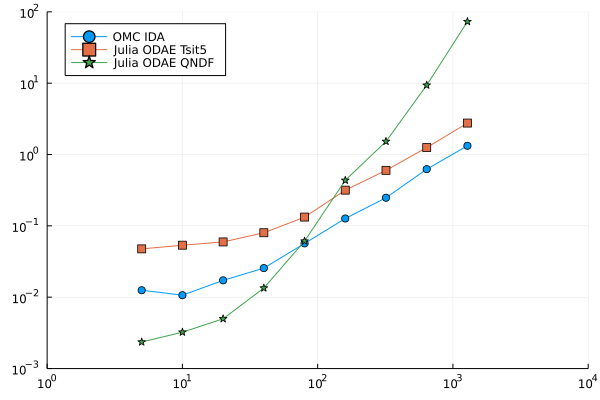
I have tried quite a bunch of options but Tsit5 and QNDF look most promising. The Tsit5() scales the same as OMC but is approximately. twice slower - > I am happy. The QNDF(autodiff=false) is quite faster for small N but scales quite bad. Why does QNDF scale this bad with N? Is there some other solvers I can try, or some other solver options etc.? (I also tried IDA() from Sundials.jl, but it was no good either.) Should I even expect to beat OMC with Julia like this?
Thank you for any response
The MTK model:
Modelica Version:
]st
[6e4b80f9] BenchmarkTools v1.3.1 [336ed68f] CSV v0.10.4 [052768ef] CUDA v3.11.0 [a93c6f00] DataFrames v1.3.4 [82cc6244] DataInterpolations v3.9.2 [39dd38d3] Dierckx v0.5.2 [aae7a2af] DiffEqFlux v1.51.2 [41bf760c] DiffEqSensitivity v6.79.0 [0c46a032] DifferentialEquations v7.2.0 [f6369f11] ForwardDiff v0.10.30 [615f187c] IfElse v0.1.1 [a98d9a8b] Interpolations v0.14.0 [ef3ab10e] KLU v0.3.0 [7f56f5a3] LSODA v0.7.0 [b964fa9f] LaTeXStrings v1.3.0 [7ed4a6bd] LinearSolve v1.20.0 [eff96d63] Measurements v2.7.2 [961ee093] ModelingToolkit v8.15.1 [7f7a1694] Optimization v3.7.1 [1dea7af3] OrdinaryDiffEq v6.18.1 [f0f68f2c] PlotlyJS v0.18.8 [91a5bcdd] Plots v1.31.2 [f27b6e38] Polynomials v3.1.4 [1fd47b50] QuadGK v2.4.2 [731186ca] RecursiveArrayTools v2.31.1 [276daf66] SpecialFunctions v2.1.7 [43dc94dd] SteamTables v1.3.0 [c3572dad] Sundials v4.9.4 [0c5d862f] Symbolics v4.9.0 [a759f4b9] TimerOutputs v0.5.20 [95ff35a0] XSteam v0.3.0
OMC OpenModelica v1.19.2