expmv and phimv performance

[ChrisRackauckas]

I think there's still some things to investigate.

1. Does this view hurt performance moreso than allocating? https://github.com/JuliaDiffEq/OrdinaryDiffEq.jl/pull/365#discussion_r190770827
2. How's the new expmv and phimv vs the ones from ExpoKit.jl. What's the performance difference and numerical stability difference? I know ExpoKit.jl does some extra stepping, so is it more numerically stable but with an extra cost? Curious to have this mapped out.

@MSeeker1340

[MSeeker1340]

So the preliminary accuracy/performance analysis comparison with Expokit is here: https://gist.github.com/MSeeker1340/5f5f9f1333824ee7aa7052b98a0e6dc2 The results are... a bit alarming, at least for big h. It seems that if the size of Krylov subspace is small then our non-subdividing implementation performs rather poorly. Of course, when you look at the performance analysis, you can see that Expokit spends much more time in the case of large h because of the subdividing. But the gap in accuracy is just too big to justify using the non-subdividing version. It turns out Expokit's approach does make sense after all. Now, say that we switch back to using Expokit's subdivision approach. Then the problem would be how to formulate a time-stepping method analogous to what Expokit does in the case of phimv to higher order phi functions. Guess it's time to start doing some algebra then.

[MSeeker1340]

I figured it might be best to use a real-life example to test the accuracy of expmv, as well as compare it with explicit RK methods.

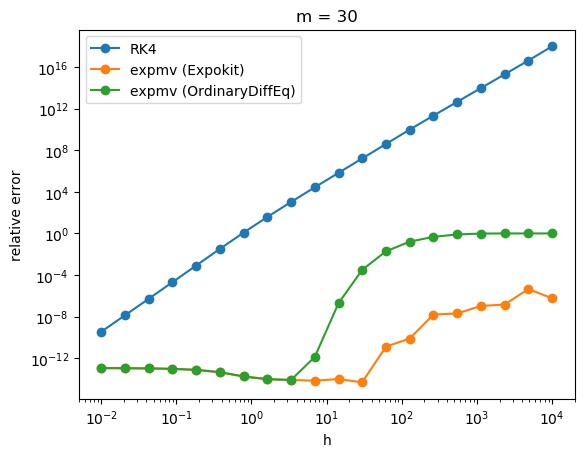
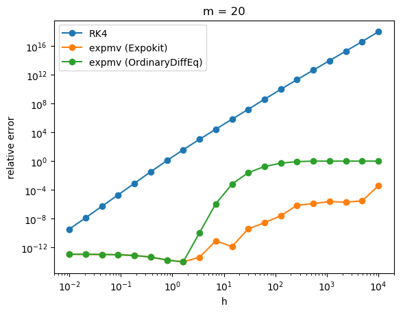
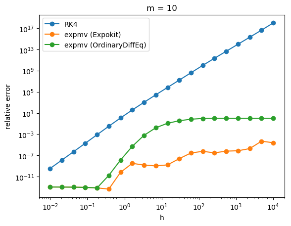
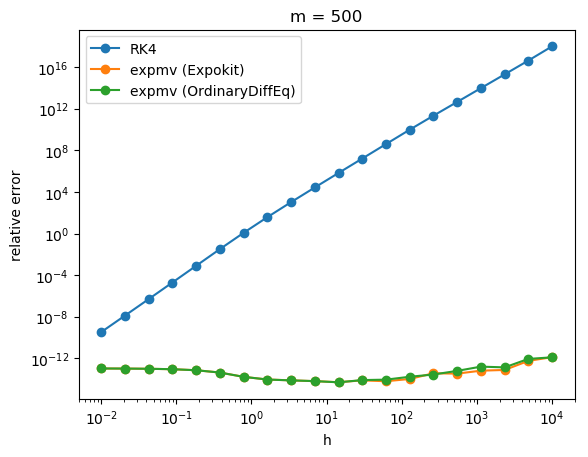
So I recorded the two versions of expmv as well as RK4's time stepping accuracy when applied to the 1D diffusion equation with central differencing discretization. The system's dimension is n = 500 and h is the Courant number dt/dx^2.

Note that these are the errors of just a single time step.

The first figure shows the full Krylov expansion case, and as can be expected both versions of expmv have high accuracy. As the subspace size m decreases, the error in expmv increases, wich Expokit's version having significantly higher accuracy for larger h.

I think what the results show is that even with OrdinaryDiffEq's less-accurate version of expmv, it still outperforms RK4 by a large margin. Also the difference between the two versions don't start to show after a certain threshold, depending on the value of m.

The verdict then should probably be something like this: for moderately large m and small h, OrdinaryDiffEq's simpler implementation should suffice. For small m and large h, Expokit's method should be preferred. However, whether the need for that would arise in real applications is debatable. (Also I still couldn't find an easy way to generalize Expokit's internal time stepping method to higher order phis).

We can also get some quick performance estimation from the figures. Ignoring overhead, if one matvec computation takes unit time, then one RK4 step takes 4 units of time and expmv takes m units of time. So for example in the case of m = 20, suppose we want to get 1e-8 accuracy, then using the expmv from OrdinaryDiffEq we can choose about 100x bigger h than RK4. Since in this case one expmv step takes 5x as much time as RK4, we should expect a 20x performance boost.

One thing of interest is how expmv seems to have an upper bound of error regardless of m. I think this is covered somewhere in literature but I have to dig a bit. Could be helpful if our phimv, etc can give out an error estimation for the integrators.

I'll do the experiments with Schrodinger's equation to test out the imaginary spectrum case and post updates here.

[ChrisRackauckas]

But ExpoKit's expmv does multiple steps so shouldn't it be more expensive than OrdinaryDiffEq's? What happen's when you factor that cost in: is it worth it?

[MSeeker1340]

I can probably fork a clone of Expokit and modify its expmv so that it returns the number of inner time stepping taken. This would be more better than, say, simple @time its performance.

[ChrisRackauckas]

Can you do a plot of error vs time? That's the most interesting performance wise. It's normally referred to as a work-precision or precision-work diagram and it tells the real practical tradeoff.

[MSeeker1340]

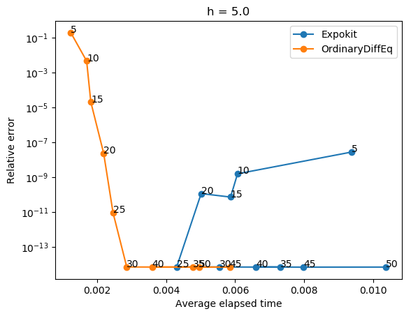
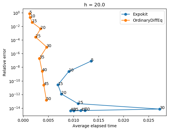
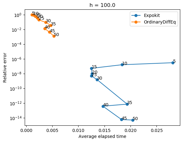
The work-precision diagrams:

Still using 1D heat equation as an example. Both non-allocating versions of expmv! are used. The annotation corresponds to the size of the Krylov subspace m.

One thing to note is that I'm still using the non-contiguous view in OrdinaryDiffEq's expmv!, so it might not be optimized. Nevertheless I think the diagrams agrees with my previous conclusion: that for relatively small h (still bigger than what RK4 allows), internal time stepping is not necessary. For large h it is significantly better though, but again the question is whether there will be a need to use such a large time step. (Doesn't hurt to include this as an option though, if we can find out how to generalize the time stepping method).

The behavior of Expokit is also interesting in itself. Because of the existence of internal time stepping, using a smaller m can actually result in more time spent on the time stepping part, unlike OrdinaryDiffEq whose behavior is simpler (there does exist some zigzags though for large h; not sure why).

Attaching plotting notebook for reference: Accuracy & Performance Analysis of expmv.pdf

[ChrisRackauckas]

I think this is good evidence that what you have is at least good for now, and internal time stepping can be added later as part of a finalizing touch, but isn't crucial.

[MSeeker1340]

To address the first question:

Here expmv2! and phimv2! are modified from expmv! and phimv! to not use non-contiguous caches but instead allocates.

The set up mirrors a usual case in application: a size 30 Krylov subspace is used, but in construction the maximum dimension is set to 50, so that results in non-contiguous caches being used in expmv! and phimv!.

using OrdinaryDiffEq: KrylovSubspace, arnoldi!, expmv!, expmv2!, phimv!, phimv2!

n = 100
K = 4
maxiter = 50
m = 30
A = randn(n, n)
b = randn(n)
Ks = KrylovSubspace{Float64}(n, maxiter)
arnoldi!(Ks, A, b; m=m);

w = zeros(n)
cache = zeros(maxiter, maxiter)
@time expmv!(w, 1.0, Ks; cache=cache);

  0.003151 seconds (63 allocations: 281.906 KiB)

@time expmv2!(w, 1.0, Ks);

  0.003148 seconds (58 allocations: 288.828 KiB)

w = zeros(n, K+1)
caches = (zeros(maxiter), zeros(maxiter, maxiter), zeros(maxiter+K, maxiter+K), zeros(maxiter, K+1))
@time phimv!(w, 1.0, Ks, K; caches=caches);

  0.000534 seconds (71 allocations: 360.469 KiB)

@time phimv2!(w, 1.0, Ks, K);

  0.000559 seconds (66 allocations: 378.047 KiB)

The timings fluctuate a bit, but they are more or less the same. Actually, the performance bottleneck of both functions seem to lie in expm, as can be demonstrated below:

H = copy(Ks[:H])
# Construct the Hk used by phimv
Hk = zeros(m+K, m+K)
e = zeros(m); e[1] = 1.0
Hk[1:m, 1:m] = H
Hk[1:m, m+1] = e
for i = m+1:m+K-1
    Hk[i, i+1] = 1.0
end

@time expm(H);

  0.003176 seconds (53 allocations: 288.625 KiB)

@time expm(Hk);

  0.000548 seconds (53 allocations: 368.750 KiB)

So it doesn't really make a difference whether we choose the non-allocating or allocating version.

It is also worth noting that expm on the larger Hk is actually faster than the smaller H. A peculiar result indeed, but I think it has something to do with Higham's scaling method and the fact that Hk has a lot of zeros.

[ChrisRackauckas]

I think it has to do with the inner contiguous buffers of most BLAS implementations, so okay cool we don't need to worry about it.

[MSeeker1340]

Cool. With these two questions answered I think what's left of the exponential utilities is error estimation.

We have dense and sparse methods that are numerically stable and maintain accuracy for not-so-large h. What we don't have is a way of estimating the error a priori. That is, a way for the integrator to choose how big m to use based on h and the linear operator.

I read somewhere on the Expokit paper that a posteriori error estimation can be achieved by computing the next order phi (this is what they used to control the internal time stepping). This too can be useful to the integrators, but a priori estimation would be best.

Think I need to dig into the literature on this one. Do you recall any paper that may be of help?

[MSeeker1340]

Forgot to mention: another thing we can improve on is the special case when the linear operator is symmetric/Hermitian. In this case the faster Lanczos algorithm can be used instead of the arnoldi iterations.

[ChrisRackauckas]

Forgot to mention: another thing we can improve on is the special case when the linear operator is symmetric/Hermitian. In this case the faster Lanczos algorithm can be used instead of the arnoldi iterations.

Good point. This is important for PDEs.

Think I need to dig into the literature on this one. Do you recall any paper that may be of help?

What does the EPIRK codes do? a priori error estimates tend to be pretty bad in comparison to posteriori error estimates, so if the next order phi isn't a costly computation then that's a good idea. Otherwise, the previous order phi could be used?

[MSeeker1340]

Before closing the issue, here's the work-precision diagrams for imaginary spectrum problems (example being 1D Schrodinger's equation). Same methodology as above:

Not really different than the real negative case. The errors are a bit worse and execution time is about 5x that of the real problem. I guess this is mostly due to complex arithmetic and linear algebra right?