Open keatonb opened 
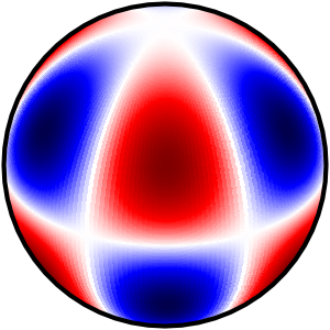
6 years ago
If you change your longitudes to be -pi -> pi rather than 0 -> 2*pi, contourf works as expected. Weird that it would work differently in the two different methods depending on the longitudes.
This is the change I made:
lon = np.linspace(0,2*np.pi,200) - np.pi
The default central longitude for PlateCarree
is 0, so I guess it makes sense that the input range should be -pi <-> pi.
Thanks for your input!
Subtracting pi did work for that particular example, but it does not fix the problem generally for other data. For instance, if I change to
lon = np.linspace(0,2*np.pi,200)-np.pi
and add
drm = -1.*drm
before plotting, I now get:
That is curious indeed! It looks like the issues arise when the drm values are close to zero. Following a suggestion from this basemap issue
drm[np.abs(drm) < 1.e-6] = 0.
Setting small values of drm to zero directly worked for me in all cases. Even with lons 0 -> 2*pi. So, my original suggestion had nothing to do with the problem it looks like. I'm still not sure why this is happening, but hope this helps you out anyways.
Yes, that does seem to work in most cases, but I have to tune that "close to zero" limit depending on the situation.
I think I actually found a simple fix: setting the contour line values explicitly instead of just specifying the number.
I have no idea why this makes a difference. Inspecting the levels
property returned in the contourf object, nothing looks odd. Things work for me when I specify those exact levels explicitly.
I'm experiencing the same on some geo data plots. In some cases (apparently casually but reproducible and linked with data resolution) the negative contourf disappear from the plots. Opening the produced pdf files with Inkscape, I found that the negative contourf are in effect produced but then hided by other levels. I'm attaching the original plot and the reconstructed one, in which I just changed the order of levels inside Inkscape. It appears to be a problem with the zorder of contourf patches..
ps. I tried outputting different filetypes, but the problem persists, and for the same datasets bug.pdf .
It's not really a zorder problem; some paths just get transformed to fill the whole area when they shouldn't.
So, I can reproduce this problem if I pass levels = np.arange(-42, 43, 2) / 100
, but not levels = np.arange(-0.42, 0.43, 0.02)
. The difference being that, due to floating point addition, in the latter case the '0' contour level is actually 3.88578059e-16. So the path is just ever so slightly different enough to not trigger the bad transform.
The '0' contour level path is generally one that fills the entire Plate Carree space (see below), with some holes cut out of it for the other contours. Because of that, I think the problem is fairly similar to #1149 and #146 as it has to do with polygons that fill the entire space and need to be stitched back together, but aren't correctly.
Well, I'm a bit confused now, because I can extract the path used to plot the 0-contour, and plot it on a new figure, and it appears fine:
cf = ax0.contourf(lon*180/np.pi, lat*180/np.pi, drm, levels,
transform=ccrs.PlateCarree(), cmap='seismic')
for i, pc in enumerate(cf.collections):
if i == 20:
path = pc.get_paths()[0]
fig1 = plt.figure()
ax1 = fig1.add_subplot(1, 1, 1, projection=ccrs.Orthographic(0, 30))
ax1.add_patch(
matplotlib.patches.PathPatch(path, transform=ccrs.PlateCarree()))
ax1.set_global()
which naturally makes it really hard to debug.
@QuLogic I think you must have had your 'levels' fix in there from before. When I use your code I get what you were saying earlier with the zero level taking up the entire area. The reason the high regions still show up is because of the drawing order. I agree with all of your assessments of related issues and clipping/patching the paths together being the issue. I don't have a solution for that though.
Here is a contained example to reproduce the issues for copy.paste purposes.
import matplotlib
import matplotlib.pyplot as plt
import numpy as np
import scipy.special as sp
import cartopy
import cartopy.crs as ccrs
# Compute spherical harmonic pattern
l=4; m=3
lon = np.linspace(0,2*np.pi,200)
lat = np.linspace(-np.pi/2,np.pi/2,500)
colat = lat+np.pi/2
d = np.zeros((len(lon),len(colat)),dtype = np.complex64)
meshed_grid = np.meshgrid(lon, lat)
lat_grid = meshed_grid[1]
lon_grid = meshed_grid[0]
for j, yy in enumerate(colat):
for i, xx in enumerate(lon):
d[i,j] = sp.sph_harm(m,l,xx,yy)
drm = np.transpose(np.real(d))
#Plot example with contour() and contourf()
fig, (ax1, ax2) = plt.subplots(1, 2, subplot_kw={'projection': ccrs.Orthographic(0, 30)})
levels = np.arange(-42, 43, 2) / 100
#levels = np.arange(-0.42, 0.43, 0.02)
#contour() works as expected
ax1.contour(lon*180/np.pi,lat*180/np.pi,drm,levels,
transform=ccrs.PlateCarree(),cmap='seismic')
ax1.relim()
ax1.autoscale_view()
#contourf() doesn't
cf = ax2.contourf(lon*180/np.pi,lat*180/np.pi,drm,levels,
transform=ccrs.PlateCarree(),cmap='seismic')
fig1 = plt.figure()
ax1 = fig1.add_subplot(1, 2, 1, projection=ccrs.Orthographic(0, 30))
ax2 = fig1.add_subplot(1, 2, 2, projection=ccrs.PlateCarree())
for i, pc in enumerate(cf.collections):
if i == 20:
path = pc.get_paths()[0]
ax1.add_patch(
matplotlib.patches.PathPatch(path, transform=ccrs.PlateCarree()))
ax1.set_global()
ax2.add_patch(
matplotlib.patches.PathPatch(path, transform=ccrs.PlateCarree()))
ax2.set_global()
@greglucas Ah right, sorry I forgot, you must copy it to make it fix itself: path = pc.get_paths()[0].deepcopy()
, which is essentially the same as saving to a file and loading again.
Hi, does someone have any news on this? I moved to the Stereographic projection to avoid the bug, but would be great to go back to the Orthographic..
I ended up using pcolormesh for my application instead of contourf to avoid this issue. Not exactly the same, but at least I can get an Orthographic projection this way.
Hi,
a short update on this. I initially thought the Stereographic would work, but actually I find the same bug (i.e. negative contourf not drawn) for the Stereographic and the Nearside projections. The bug appears very often (more than 50% of the cases) when a contourf is crossing the 0 value, which makes that contourf spread to cover the full image. It does not appear when 0 is one of the levels.
I think this is a very serious bug. This makes it impossible to reliably produce filled contours when looking at the poles. Is there a timeline for solving this? It has been more than one year now..
@fedef17 If you can reduce down to a self-contained example that reproduces the problem, that would be helpful. We have one of those above, but it would be good to collect several, since I'm sure we're dealing with edge cases in the current algorithm.
It seems that the issue described in the first example can be managed by the workaround presented in issue #1421 as this seems to be a case of overlapping data.
The results obtained with the code below:
import matplotlib.pyplot as plt
import numpy as np
import numpy.ma as ma
import scipy.special as sp
import cartopy.crs as ccrs
def z_masked_overlap(axe, X, Y, Z, source_projection=None):
"""
for data in projection axe.projection
find and mask the overlaps (more 1/2 the axe.projection range)
X, Y either the coordinates in axe.projection or longitudes latitudes
Z the data
operation one of 'pcorlor', 'pcolormesh', 'countour', 'countourf'
if source_projection is a geodetic CRS data is in geodetic coordinates
and should first be projected in axe.projection
X, Y are 2D same dimension as Z for contour and contourf
same dimension as Z or with an extra row and column for pcolor
and pcolormesh
return ptx, pty, Z
"""
if not hasattr(axe, 'projection'):
return X, Y, Z
if not isinstance(axe.projection, ccrs.Projection):
return X, Y, Z
if len(X.shape) != 2 or len(Y.shape) != 2:
return X, Y, Z
if (source_projection is not None and
isinstance(source_projection, ccrs.Geodetic)):
transformed_pts = axe.projection.transform_points(
source_projection, X, Y)
ptx, pty = transformed_pts[..., 0], transformed_pts[..., 1]
else:
ptx, pty = X, Y
with np.errstate(invalid='ignore'):
# diagonals have one less row and one less columns
diagonal0_lengths = np.hypot(
ptx[1:, 1:] - ptx[:-1, :-1],
pty[1:, 1:] - pty[:-1, :-1]
)
diagonal1_lengths = np.hypot(
ptx[1:, :-1] - ptx[:-1, 1:],
pty[1:, :-1] - pty[:-1, 1:]
)
to_mask = (
(diagonal0_lengths > (
abs(axe.projection.x_limits[1]
- axe.projection.x_limits[0])) / 2) |
np.isnan(diagonal0_lengths) |
(diagonal1_lengths > (
abs(axe.projection.x_limits[1]
- axe.projection.x_limits[0])) / 2) |
np.isnan(diagonal1_lengths)
)
# TODO check if we need to do something about surrounding vertices
# add one extra colum and row for contour and contourf
if (to_mask.shape[0] == Z.shape[0] - 1 and
to_mask.shape[1] == Z.shape[1] - 1):
to_mask_extended = np.zeros(Z.shape, dtype=bool)
to_mask_extended[:-1, :-1] = to_mask
to_mask_extended[-1, :] = to_mask_extended[-2, :]
to_mask_extended[:, -1] = to_mask_extended[:, -2]
to_mask = to_mask_extended
if np.any(to_mask):
Z_mask = getattr(Z, 'mask', None)
to_mask = to_mask if Z_mask is None else to_mask | Z_mask
Z = ma.masked_where(to_mask, Z)
return ptx, pty, Z
# Compute spherical harmonic pattern
l=4; m=3
lon = np.linspace(0,2*np.pi,200)
lat = np.linspace(-np.pi/2,np.pi/2,500)
colat = lat+np.pi/2
d = np.zeros((len(lon),len(colat)),dtype = np.complex64)
meshed_grid = np.meshgrid(lon, lat)
lat_grid = meshed_grid[1]
lon_grid = meshed_grid[0]
for j, yy in enumerate(colat):
for i, xx in enumerate(lon):
d[i,j] = sp.sph_harm(m,l,xx,yy)
drm = np.transpose(np.real(d))
#Plot example with contour() and contourf()
fig, ((ax1, ax2), (ax3, ax4)) = plt.subplots(2, 2,
subplot_kw={'projection': ccrs.Orthographic(0, 30)})
#contour() works as expected
ax1.contour(lon*180/np.pi,lat*180/np.pi,drm,51,
transform=ccrs.PlateCarree(),cmap='seismic')
ax1.relim()
ax1.autoscale_view()
#contourf() doesn't
ax2.contourf(lon*180/np.pi,lat*180/np.pi,drm,51,
transform=ccrs.PlateCarree(),cmap='seismic')
ax2.relim()
ax2.autoscale_view()
lons, lats = np.meshgrid(lon*180/np.pi, lat*180/np.pi)
# mask the overlaps
X, Y, masked_drm = z_masked_overlap(
ax4, lons, lats, drm,
source_projection=ccrs.Geodetic())
ax3.contour(X ,Y ,masked_drm, 51,
cmap='seismic')
ax3.relim()
ax3.autoscale_view()
ax3.set_title('after z_masked_overlap workaround')
ax4.contourf(X ,Y ,masked_drm, 51,
cmap='seismic')
ax4.relim()
ax4.autoscale_view()
ax4.set_title('after z_masked_overlap workaround')
plt.tight_layout()
plt.savefig('img/sphericalcontours.png')
@fedef17 If you can reduce down to a self-contained example that reproduces the problem, that would be helpful. We have one of those above, but it would be good to collect several, since I'm sure we're dealing with edge cases in the current algorithm.
Hi @dopplershift, here is a self-contained example from my work to reproduce the problem. I agree with previous comments that this is rather serious from a user's perspective, and it would be good to fix it soon. I don't have the expertise to debug cartopy but I'm happy to help where I can.
For me the problem only occurs under the following conditions:
I have tested with cartopy version 0.18.0b1.
Below the plot demonstrating the problem together with the code that produces the plot. Data file (~200kB, NetCDF4) is attached.
import matplotlib.pyplot as plt
import xarray as xr
import cartopy
import cartopy.crs as ccrs
from cartopy.util import add_cyclic_point
# load data
fig = plt.figure(figsize=(12, 4))
da = xr.open_dataarray('testdata.nc')
lats = da.latitude.values
lons_nocyclic = da.longitude.values
data_nocyclic = da.values
data, lons = add_cyclic_point(da.values, coord=lons_nocyclic)
# negative contours not shown for these contour levels
nok_levels = [-0.4, -0.2, 0.2, 0.4]
# negative contours are correctly shown for these contour levels
ok_levels = [-.4, -.3, -0.2, -0.1, 0.1, 0.2, .3, .4]
# keyword arguments for contourf and colorbar
conargs = dict(transform=ccrs.PlateCarree(), cmap='RdBu_r', extend='both')
cbargs = dict(orientation='horizontal', pad=0.05, extend='both')
# 1) problem: negative contours not shown
plt.subplot(1, 3, 1, projection=ccrs.NorthPolarStereo())
c1 = plt.contourf(lons, lats, data, nok_levels, **conargs)
plt.colorbar(c1, **cbargs)
plt.title('(a) missing negative contours')
# 2) problem disappears with slightly different contour levels
plt.subplot(1, 3, 2, projection=ccrs.NorthPolarStereo())
c2 = plt.contourf(lons, lats, data, ok_levels, **conargs)
plt.colorbar(c2, **cbargs)
plt.title('(b) change levels: no problem')
# 3) problem disappears with slightly different contour levels
plt.subplot(1, 3, 3, projection=ccrs.NorthPolarStereo())
c3 = plt.contourf(lons_nocyclic, lats, data_nocyclic, nok_levels, **conargs)
plt.colorbar(c3, **cbargs)
plt.title('(c) no cyclic point: no problem')
# add decorations to plots and save
for ax in plt.gcf().axes:
if type(ax) == cartopy.mpl.geoaxes.GeoAxesSubplot:
ax.set_extent((-180.0, 180.0, 45.0, 90.0), ccrs.PlateCarree())
ax.gridlines()
ax.coastlines()
fig.savefig('cartopy_test.png')
I think that last problem should be fixed by @htonchia's idea here, though I'm not sure it'll fix the original problem.
I also came across this problem recently. Here's another example that reproduces it:
import numpy as np
import matplotlib.pyplot as plt
import cartopy.crs as ccrs
N = 10
state = np.random.RandomState(23)
fig = plt.figure(figsize=(5, 2.5))
ax = fig.add_subplot(projection=ccrs.Mollweide())
ax.coastlines()
x = np.linspace(-180, 180, N)
y = np.linspace(-90, 90, N)
z = state.rand(N, N) * 10 - 5
m = ax.contourf(
x, y, z,
transform=ccrs.PlateCarree(),
cmap='RdBu_r',
vmin=-5,
vmax=5,
)
fig.colorbar(m, ax=ax)
And the resulting output:
It seems to depend on the figure size, dataset, and projection -- sometimes the problem appears, sometimes it doesn't. I had to randomly try different np.random.RandomState
seeds to generate this result. Very very strange.
I've just come across this too, in cartopys 0.17, 0.18, 0.20.1.
My code: (the data file temp.nc is in the attached temp.zip)
import numpy as np
import cartopy
import cartopy.crs as ccrs
import iris
import iris.quickplot as qplt
import matplotlib.pyplot as plt
mycube = iris.load_cube("temp.nc")
proj = ccrs.Orthographic(central_longitude=0.0, central_latitude=90.0)
# This works correctly (Figure 1):
qplt.contourf(mycube,np.linspace(-9,0,11),axes=plt.axes(projection=proj)) ; qplt.plt.gca().coastlines() ; qplt.show()
# This plots incorrectly (Figure 2):
qplt.contourf(mycube,np.linspace(-9,0,10),axes=plt.axes(projection=proj)) ; qplt.plt.gca().coastlines() ; qplt.show()
# There is no problem on the Plate Carree projection:
qplt.contourf(mycube,np.linspace(-9,0,11)) ; qplt.plt.gca().coastlines() ; qplt.show()
qplt.contourf(mycube,np.linspace(-9,0,10)) ; qplt.plt.gca().coastlines() ; qplt.show()
# Also works without iplt: (thanks @rcomer !)
axes = plt.axes(projection=proj)
plt.contourf(
mycube.coord("longitude").points,
mycube.coord("latitude").points,
mycube.data,
levels=np.linspace(-9, 0, 10),
transform=ccrs.PlateCarree(),
)
axes.coastlines()
plt.colorbar(orientation="horizontal")
plt.show()
Plots:
If I make Figure 2 as a svg and load it into Inkscape, I can confirm that the other contour levels are present, just underneath the zero-layer.
In my case, setting the cube data values near zero to be exactly zero doesn't help;
and np.linspace(-9,0,11)
and np.linspace(-9,0,10)
both seem to have zeros at exactly zero (rather than somethingE-16)
I am currently having this issue in Cartopy 0.21.1. Here is my code:
import numpy as np
import math
import csv
import matplotlib.pyplot as plt
import cartopy.crs as ccrs
import cartopy.feature as cf
resY = 360
resX = 720
extent_globe = np.radians([0,360,-90,90])
grid_lon = np.linspace(extent_globe[0], extent_globe[1], resX)
grid_lat = np.linspace(extent_globe[2], extent_globe[3], resY)
grid_lons, grid_lats = np.meshgrid(grid_lon, grid_lat)
part1 = np.square(np.tan(math.pi / 3)) / np.square(np.tan(grid_lats))
btheta = np.where(grid_lats > 0, part1 * np.exp(1 - part1), 0)
cpart = 0.6 * 2 * math.pi * np.cos(1 * grid_lons)
forcing = btheta * cpart
fig = plt.figure()
ax1 = plt.subplot(projection=ccrs.Orthographic(central_latitude=90))
cs = ax1.contourf(np.rad2deg(grid_lons), np.rad2deg(grid_lats), forcing, cmap='RdBu_r', transform=ccrs.PlateCarree(), levels=np.mgrid[-10:10:21j])
plt.title(f'Wavenumber 1 Forcing')
cbar = fig.colorbar(cs)
plt.show()
In this case, it shows the negative contours if I replace forcing
with -forcing
, but if I replace np.cos(1 * grid_lons)
with np.cos(2 * grid_lons)
then the negative sign does not reveal the negative contours. The previously suggested solutions of changing the longitude range to be 0 to 360 and zeroing out small values did not fix the error.
Description
I'm trying to draw spherical harmonic contours on an orthographic projection of a sphere. I see the correct contours when calling contour(), but many are not filled by contourf(). I think this is a bug, perhaps related to Issue 1024 (but I couldn't view their example figures).
Code to reproduce
Traceback
No error reported.
Full environment definition
### Operating system OS X 10.10.5 ### Cartopy version 0.16.0 ### conda list ``` # packages in environment at /Users/keatonb/anaconda: # # Name Version Build Channel _license 1.1 py27_0