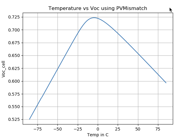
 After adding Isat2 dependance on Tcell same as Isat1
Closed mikofski closed 6 years ago
 After adding Isat2 dependance on Tcell same as Isat1
Wow! looks great!!! You are awesome!!! 🎉 🏅 🌈 🦄
The generated coefficients are a much better fit to the IV curves now at all irradiance and temperatures!

@BenBourne , also, I am now able to fit the entire IEC-61853 test matrix and the results are very good, even better than the STC only generated coefficients!

Nice work, Chetan!
This issue is addressed in v4.0 but needs further work to match close with the data sheet coefficients. Going to leave the issue open till we have validation work complete on this issue.
On the issue of MPP vs. temperature, @mikofski any idea why this behavior is observed?

Hi @rayhickey, Sorry, I'm not sure what I'm seeing. Can you please give me more detail? Thanks! -m
These are maximum power points on 2-Diode modeled I-V curves from PVMismatch at steps of 1 degree C. I'm not sure if this is the expected behavior of I-V curves as a function of temperature, but I_mp follows a cyclical trend that spans every ~11 degrees, followed by a large discontinuity. V_mp has similar discontinuities, though still decreases monotonically. Does this seem like it would have a physical basis? Chetan suggested there could be some floor division happening but importing future division didn't fix it.


@rayhickey how are you obtaining Imp and Vmp?
I think what's happening is that you are using the PVsystem method calcMPP_IscVocFFeff and pvconst.npts is too small, the default is 101, so you are seeing a jump from one discrete point to the next as you traverse temperature. If you look closely at lines: 95-99 in pvsystem.py you can see that it just takes the maximum point from the calculated IV curve, it doesn't interpolate to find a better guess.
We had tried to improve this, but there was an issue #9 (fixed in 623adb8e8259b13c40c8b043f18bef3ec04599cc specifically the diff of pvsystem.py) so we scrapped it, and just decided to increase the number of IV points as needed to like 1001, but even that is still discrete, so there are deltas as the max value jumps from point to point. We didn't want to lock the user into a large number of IV curve points so we left the default at 101, but probably should have added something to the documentation.
I think that this deserves revisiting. If the issue in #9 was that the search window was too big, just decrease it since we know the index where the mpp is, just choose a point to the left and a point to the right.
mpp = np.argmax(self.Psys)  # index near MPP

# get points just to the left and right of mpp
P = self.Psys[mpp-1:mpp+1, 0]
V = self.Vsys[mpp-1:mpp+1, 0]
I = self.Isys[mpp-1:mpp+1, 0]

# calculate derivative dP/dV using central difference
dP = np.diff(P, axis=0)  # size is (2, 1)
dV = np.diff(V, axis=0)  # size is (2, 1)
Pv = dP / dV  # size is (2, 1)

# dP/dV is central difference at midpoints,
Vmid = (V[1:] + V[:-1]) / 2.0  # size is (2, 1)
Imid = (I[1:] + I[:-1]) / 2.0  # size is (2, 1)

# interpolate to find Vmp
Vmp = -Pv[0] * np.diff(Vmid, axis=0) / np.diff(Pv, axis=0) + V[0]
Imp = -Pv[0] * np.diff(Imid, axis=0) / np.diff(Pv, axis=0) + I[0]
# calculate max power at Pv = 0
Pmp = Imp * Vmp
But I also think linear interpolation might be simple, and I think it's possible this approach will always just return the original maximum found. I think this is perfect for cubic interpolation because if you think of the derivative dP/dV it looks like an inverse of a 3rd order polynomial.
mpp = np.argmax(self.Psys)  # index near MPP

# just get a few points to the left and right of mpp
P = self.Psys[mpp-4:mpp+4, 0]  # size is (9, 1)
V = self.Vsys[mpp-4:mpp+4, 0]
I = self.Isys[mpp-4:mpp+4, 0]

# calculate derivative dP/dV using central difference
dP = np.diff(P, axis=0)  # size is (8, 1)
dV = np.diff(V, axis=0)
Pv = dP / dV

# dP/dV is central difference at midpoints,
Vmid = (V[1:] + V[:-1]) / 2.0  # size is (8, 1)

# shape of V vs Pv is an inverse cubic
pPv = np.polyfit(Pv, Vmid, 3)  # polynomial of Vmid(Pv)

# interpolate to find Vmp where Pv = 0
Vmp = np.polyval(pPv, 0)

# the shape of V vs P is parabolic
pP = np.polyfit(V, P, 2)  # polynomial P(V)

# interpolate to find Pmp where V = Vmp
Pmp = np.polyfit(pP, Vmp)

# calculate Imp
Imp = Pmp / Vmp
Or I think you could have used one of the stock search methods in SciPy optimize like brentq and limit the range to zero and Voc or fminbound. Note that optimization methods take functions, like a polynomial for example, and also note that brentq finds roots, while fminbound finds the minimum.
@mikofski Nice fix, it looks like the linear fit actually handles the discontinuity better than cubic interpolation. This is still just with 101 points.


Can you put together a PR? Thanks!
Well since the linear works well it and is simplest I'd go with that, but I though of another, you could just use the parabola and solve for dP/dV = 0
mpp = np.argmax(self.Psys)  # index near MPP

# just get a few points to the left and right of mpp
P = self.Psys[mpp-3:mpp+3, 0]  # size is (7, 1)
V = self.Vsys[mpp-3:mpp+3, 0]
I = self.Isys[mpp-3:mpp+3, 0]

# the shape of V vs P is roughly parabolic
p = np.polyfit(V, P, 2)  # polynomial P(V)
pder = np.polyder(p)  # polynomial of dP/dV

# calculate Vmp where pder is zero
a, b = pder  # pder = ax + b so at zero x = -b/a
Vmp = -b/a

# calculate Pmp
Pmp = np.polyval(p, Vmp)

# calculate Imp
Imp = Pmp / Vmp@rayhickey when you submit your PR please make sure to add your name to AUTHORS - ditto for you too @chetan201
Addressed in #67 and #68
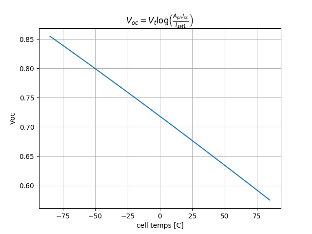
Problem: A plot of Voc vs. cell temperature shows decreasing below about zero degrees.
Should look like this
Possibly the lack of temperature dependence of Isat2 is the culprit?
Proposed: Use cubic temperature dependence for Isat2 same as for Isat1.
addressed in #64