 YuVirtonomy
commented
2 months ago
YuVirtonomy
commented
2 months ago @ShuoguoZhangTUM can you check this issue?
Open YuVirtonomy opened 2 months ago
YuVirtonomy
commented
2 months ago @ShuoguoZhangTUM can you check this issue?
 ShuoguoZhangTUM
commented
2 months ago
ShuoguoZhangTUM
commented
2 months ago @ShuoguoZhangTUM can you check this issue?
show me the equation about how you calculate the mu_f and U_f. Maybe you calculate these two parameters wrongly
YuVirtonomy
commented
2 months ago @ShuoguoZhangTUM can you check this issue?
show me the equation about how you calculate the mu_f and U_f. Maybe you calculate these two parameters wrongly
$\Delta p = \frac{8 \pi \mu L Q }{A^2}$
$Q = U{avg} * A $
$U{avg} = \frac{\Delta p R^2}{8\mu L}$
ShuoguoZhangTUM
commented
2 months ago @ShuoguoZhangTUM can you check this issue?
show me the equation about how you calculate the mu_f and U_f. Maybe you calculate these two parameters wrongly
Δp=8πμLQA2 Q=Uavg∗A Uavg=ΔpR28μL
choose the max velocity as U_f, not the average velocity. Then take the max velocity into the definition of Renold number to get the mu_f. The Renold number should be prescribed by yourself
YuVirtonomy
commented
2 months ago In the most scenario, its seem more make sense to define viscosity than Reynolds number. As this is hagen flow, it is possible to obtain an analytical solution when the flow is laminar. Where the velocity profile is: $u(r) = \frac{\Delta P}{4\mu L} (R^2 - r^2)$ And the flowrate can be calculated as: $Q = A \cdot u{\text{avg}} = \int{0}^{R} 2\pi r \left( \frac{\Delta P}{4\mu L} (R^2 - r^2) \right) dr$ $A \cdot u{\text{avg}} = \pi R^2 \left( \frac{U{\text{max}}}{2} \right)$ $A*u{avg} = A \frac{U{max}}{2}$
Therefore, $u{avg} = \frac{U{max}}{2}$
As $\Delta p = \frac{8 \pi \mu L Q }{A^2} = \frac{8 \pi \mu L u{avg} A }{A^2}$, $u{avg}$ can be defined as $u_{avg} = \frac{\Delta p R^2}{8\mu L}$
The current set up in the case is set to $\Delta p = 5$, and viscousity $\mu = 3.5e-3$. while L is set to $7.5D$ With this set up, we suppose to get the result that $u{avg} =0.0377976$ and $u{max} =0.0755952$. However, its seem the velocity is way less than what we expected
!The Umax prescribed in code is maximum velocity in system, not equal to $U{max} of fluid profile
https://www.sciencedirect.com/topics/engineering/hagen-poiseuille-equation
ShuoguoZhangTUM
commented
2 months ago In the most scenario, its seem more make sense to define viscosity than Reynolds number. As this is hagen flow, it is possible to obtain an analytical solution when the flow is laminar. Where the velocity profile is: u(r)=ΔP4μL(R2−r2) And the flowrate can be calculated as: Q=A⋅uavg=∫0R2πr(ΔP4μL(R2−r2))dr A⋅uavg=πR2(Umax2) A∗uavg=AUmax2 Therefore, uavg=Umax2 As Δp=8πμLQA2=8πμLuavgAA2, uavg can be defined as uavg=ΔpR28μL The current set up in the case is set to Δp=5, and viscousity μ=3.5e−3. while L is set to 7.5D With this set up, we suppose to get the result that uavg=0.0377976 and umax=0.0755952. However, its seem the velocity is way less than what we expected !The Umax prescribed in code is maximum velocity in system, not equal to $U{max} of fluid profile
https://www.sciencedirect.com/topics/engineering/hagen-poiseuille-equation
I put your physical and geometric parameters into my 3-D hagen flow, i get the exactly same velocity profile as the analytical solution. I already checked your code, and you wrongly modified the code how to impose boudary pressure, etc. Please create 3D flow according to the upload test 2D flow. You just need to modify the 2D geometry body into 3D, and use the Rotation3d for the trasformation.
Attention, dont modify anything eles, especially the class about the bidirectional buffer and how to impose pressure here it my parameter setting in 3D hagen flow according to your code
 Xiangyu-Hu
commented
2 months ago
Xiangyu-Hu
commented
2 months ago @YuVirtonomy How about the result?
YuVirtonomy
commented
2 months ago This case is built on the test_2d_pulsatile_poiseuille_flow. It seems you've defined the resolution as resolution_ref = radius/10.
The difference is in test_2d_pulsatile_poiseuille_flow: in LeftBidirectionalBufferCondition & RightBidirectionalBufferCondition, you declared Real pressure = Inlet_pressure & Real pressure = outlet_pressure in getTargetPressure.
Whereas, I've implemented an inletpressure member in my BidirectionalBufferCondition class and initialized the value according to inlet and outlet pressure. In getTargetPressure, a function compute_pressure is deployed to update the target_pressure according to runtime if necessary. In the current case, compute_pressure does nothing other than directly feedback the pressure.
The same applies to LeftInflowPressure & RightInflowPressure in test_2d_pulsatile_poiseuille_flow and the InflowPressure in the current case.
I've also tried your way of declaring both LeftBidirectionalBufferCondition, RightBidirectionalBufferCondition, LeftInflowPressure, and RightInflowPressure. It seems the results are exactly the same.
The result of the simulation with a resolution equal to diameter / 10 is shown in the image. The velocity in the radial direction is based on the observer deployed at half the length. Here is a summary:
This result is the simulation with a resolution equal to diameter / 10. The velocity is obtained through observers located at (length * 0.5, 0, Z). Maximum velocity of analytical: 0.0378 Maximum velocity of N20_no_offset: 0.0343, where the pressure is set to 5 at the inlet and 0 at the outlet. (resolution equal to diameter / 20) Maximum velocity of N10_no_offset: 0.0306, where the pressure is set to 5 at the inlet and 0 at the outlet Maximum velocity of N10_offset: 0.0277, where the pressure is set to 10 at the inlet and 5 at the outlet Maximum velocity of N10_no_offset_PinVout: 0.0373, where the pressure is set to 5 at the inlet and 0 at the outlet
I see some major problems,
@ShuoguoZhangTUM can you please provide your full code of 3d flow in this branch and provide the cross-section velocity result?
Xiangyu-Hu
commented
2 months ago @YuVirtonomy could you also show pressure profile?
YuVirtonomy
commented
2 months ago @YuVirtonomy could you also show pressure profile?
This is the pressure profile in the axial direction
This is the velocity in the axial direction
ShuoguoZhangTUM
commented
2 months ago @YuVirtonomy could you also show pressure profile?

This is the pressure profile in the axial direction

This is the velocity in the axial direction
Xiangyu-Hu
commented
2 months ago @ShuoguoZhangTUM we should continue this pull request until the corrected obtained.
ShuoguoZhangTUM
commented
2 months ago When i use resolution=D/10, i get the same max velocity around 0.06 as your result. When i change it to D/20, the max velocity is almost same to the analytical solution. So i suggest you try higher resolution.Furthermore, my 3D flow code is same to the 2D flow code. The only difference is the parameter setting. So again, i suggest you to make your 3D flow code same as the 2D . because I can not make sure where the bug is, if you change the code too much
YuVirtonomy
commented
2 months ago I uploaded the code based on LeftBidirectionalBufferCondition, RightBidirectionalBufferCondition, LeftInflowPressure and RightInflowPressure classes.
however, I still observe the same result.
And, it can not explain why with adding an offset pressure to both inlet and outlet, the difference between the analytical solution and simulation result increases.
Also, with pressure inlet and velocity outlet, the difference between the analytical solution and simulation result decreases.
Xiangyu-Hu
commented
2 months ago @YuVirtonomy @ShuoguoZhangTUM we may need to arrange an online meeting on this issue.
I uploaded the code based on LeftBidirectionalBufferCondition, RightBidirectionalBufferCondition, LeftInflowPressure and RightInflowPressure classes.
however, I still observe the same result.
And, it can not explain why with adding an offset pressure to both inlet and outlet, the difference between the analytical solution and simulation result increases.
Also, with pressure inlet and velocity outlet, the difference between the analytical solution and simulation result decreases.
Do you have results at resolution of D/20?
Xiangyu-Hu
commented
2 months ago @YuVirtonomy @ShuoguoZhangTUM I suggest that we arrange a online meeting on this.
ShuoguoZhangTUM
commented
2 months ago @YuVirtonomy @ShuoguoZhangTUM I suggest that we arrange a online meeting on this.
Ok I also think a online meeting is very necessary
YuVirtonomy
commented
2 months ago @YuVirtonomy @ShuoguoZhangTUM I suggest that we arrange a online meeting on this.
Ok I also think a online meeting is very necessary
Could you check your email? Thanks
YuVirtonomy
commented
2 months ago 22b59063ba1963aa6826382367e75b48ca977852
Velocity measure at X (axial) direction
Short_offset & Short_no_offset: Real CR = 0.0005; /*< Channel radius. / Real CL = CR 2 4; /*< Channel length. /
Long_offset & Long_no_offset: Real CR = 0.0005; /*< Channel radius. / Real CL = CR 2 15; /*< Channel length. /
$Q = \frac{\pi r^4 \Delta P}{8 \mu L} = U{\text{max}} \times \frac{A}{2}$ $U{\text{max}} = \frac{r^2 \Delta P}{4 \mu L}$ $Re = \frac{\rho U_{\text{max}} \times 2r}{\mu}$ $\mu = \sqrt{\frac{\rho 2r^3 \Delta P}{4LRe}}$
Real mu_f = sqrt(2 rho0_f pow(CR, 3.0) fabs(Inlet_pressure - Outlet_pressure) / (4.0 Re * CL)); // using max velocity
 WeiyiVirtonomy
commented
1 month ago
WeiyiVirtonomy
commented
1 month ago Something irrelevant: the entries in particles_->sorted_id_ are not correct after adding memory buffer particles to real particles. You can look at the check_id function in test_3d_pressure_driven_poiseuille.
I know this is unrelated to the simulation since we never use the vector sorted_id_, but I think it would be better if you could always keep consistency between the index and sorted_id_.
I have added two lines to fix this issue in BidirectionalBuffer::Injection (commented out at the moment):
        size_t last_unsorted_index = particles_->unsorted_id_[particles_->total_real_particles_];
        particles_->sorted_id_[last_unsorted_index] = particles_->total_real_particles_;
You can uncomment them if you feel that it's necessary to solve this problem.
left_pressure = 5.0; right_pressure = 0.0; delta_p = left_pressure - right_pressure; mu_f = 3.5e-3; Analytical solution of velocity: U_f = delta_p radius radius / (8 full_length mu_f); U_f = 0.0377976 Reynolds number = 144.009 result: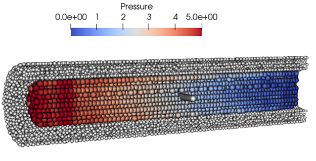
velocity at middle of axial in radial direction
The velocity magnitude is about 20% lower than the analytical solution If offset the pressure left_pressure = 20.0; right_pressure = 15.0;
Then the maximum velocity decrease even more
velocity at middle of axial in radial direction (P_in = 20, P_out = 15)