Problem with applying warps to data

[m-petersen]

Hi again,

I am facing a follow-up problem to a previous issue (https://github.com/amarquand/PCNtoolkit/issues/114) with regard to the warping process. As noted there, I have amended my code as recommended by adding "warp='WarpSinArcsinh', warp_reparam= True" to the estimate function to perform warped BLR.

My aim with this analysis is to get centile curves of WMH and related markers as well as respective z-scores for downstream predictive modelling in a sample from two cohorts.

Currently I am trying to reproduce the centile curves for WMH volume with warped BLR as presented in this manuscript (https://www.sciencedirect.com/science/article/pii/S1053811921009873#fig0004) as it accounts for potential non-gaussianity in the data. Therefore, I am following this tutorial "https://github.com/predictive-clinical-neuroscience/PCNtoolkit-demo/blob/main/tutorials/BLR_protocol/transfer_pretrained_normative_models.ipynb". The tutorials mentions that the predictions (yhat, S2) from the dummy model are after the prediction in the warped space and need to be inversely warped to achieve plotting in input space. Apparently, also the true data (y_te) is rescaled in the tutorial.

import pickle
from pcntoolkit.normative import evaluate
import matplotlib.pyplot as plt

import seaborn as sns
sns.set(style='whitegrid')

# random jitter function
def rand_jitter(arr):
    stdev = .005 * (max(arr) - min(arr))
    return arr + np.random.randn(len(arr)) * stdev

for idp_num, c in enumerate(feature_columns):

    if c in tracts_wo_wmh: continue
    print('Running IDP', idp_num, c, ':')
    roi_path = rois_path/c
    os.chdir(roi_path)

    # load the true data points
    X_te = np.loadtxt(os.path.join(roi_path, 'cov_bspline.txt'))
    yhat_te = np.loadtxt(os.path.join(roi_path, 'yhat_estimate.txt'))[:, np.newaxis]
    s2_te = np.loadtxt(os.path.join(roi_path, 'ys2_estimate.txt'))[:,np.newaxis]
    y_te = np.loadtxt(os.path.join(roi_path, f'resp_{c}.txt'))[:,np.newaxis]

    # set up the covariates for the dummy data
    print('Making predictions with dummy covariates (for visualisation)')
    yhat, s2 = ptk.normative.predict(cov_file_dummy, 
                       alg = 'blr', 
                       respfile = None, 
                       model_path = os.path.join(roi_path,'Models'), 
                       binary=False,
                       outputsuffix = '_dummy',
                       saveoutput = True,
                       warp="WarpSinArcsinh",
                       warp_reparam=True)

    # load the normative model
    with open(os.path.join(roi_path,'Models', 'NM_0_0_estimate.pkl'), 'rb') as handle:
        nm = pickle.load(handle) 

   # get the warp and warp parameters
    W = nm.blr.warp
    warp_param = nm.blr.hyp[1:nm.blr.warp.get_n_params()+1] 

    # first, we warp predictions for the true data and compute evaluation metrics
    med_te = W.warp_predictions(np.squeeze(yhat_te), np.squeeze(s2_te), warp_param)[0]
    med_te = med_te[:, np.newaxis]
    print('metrics:', evaluate(y_te, med_te))

    # then, we warp dummy predictions to create the plots
    med, pr_int = W.warp_predictions(np.squeeze(yhat), np.squeeze(s2), warp_param)

    # extract the different variance components to visualise
    beta, junk1, junk2 = nm.blr._parse_hyps(nm.blr.hyp, X_dummy)
    s2n = 1/beta # variation (aleatoric uncertainty)
    s2s = s2-s2n # modelling uncertainty (epistemic uncertainty)

    # plot the data points
    y_te_rescaled_all = np.zeros_like(y_te)
    for sid, site in enumerate(site_ids_te):
        # plot the true test data points 
        if all(elem in site_ids_tr for elem in site_ids_te):
            # all data in the test set are present in the training set

            # first, we select the data points belonging to this particular sex and site
            idx = np.where(np.bitwise_and(X_te[:,2] == sex, X_te[:,sid+len(cols_cov)+1] !=0))[0]
            if len(idx) == 0:
                print('No data for site', sid, site, 'skipping...')
                continue

            # then directly adjust the data
            idx_dummy = np.bitwise_and(X_dummy[:,1] > X_te[idx,1].min(), X_dummy[:,1] < X_te[idx,1].max())
            y_te_rescaled = y_te[idx] - np.median(y_te[idx]) + np.median(med[idx_dummy])
        else:
            # we need to adjust the data based on the adaptation dataset 

            # first, select the data point belonging to this particular site
            idx = np.where(np.bitwise_and(X_te[:,2] == sex, (df_te['site'] == site).to_numpy()))[0]

            # load the adaptation data
            y_ad = load_2d(os.path.join(idp_dir, 'resp_ad.txt'))
            X_ad = load_2d(os.path.join(idp_dir, 'cov_bspline_ad.txt'))
            idx_a = np.where(np.bitwise_and(X_ad[:,2] == sex, (df_ad['site'] == site).to_numpy()))[0]
            if len(idx) < 2 or len(idx_a) < 2:
                print('Insufficent data for site', sid, site, 'skipping...')
                continue

            # adjust and rescale the data
            y_te_rescaled, s2_rescaled = nm.blr.predict_and_adjust(nm.blr.hyp, 
                                                                   X_ad[idx_a,:], 
                                                                   np.squeeze(y_ad[idx_a]), 
                                                                   Xs=None, 
                                                                   ys=np.squeeze(y_te[idx]))
        plot the (adjusted) data points
        y_te_rescaled[y_te_rescaled < 0] = 0
        plt.scatter(rand_jitter(X_te[idx,1]), y_te_rescaled, s=4, color=clr, alpha = 0.1)

    # plot the median of the dummy data
    plt.plot(xx, med, clr)

    # fill the gaps in between the centiles
    junk, pr_int25 = W.warp_predictions(np.squeeze(yhat), np.squeeze(s2), warp_param, percentiles=[0.25,0.75])
    junk, pr_int95 = W.warp_predictions(np.squeeze(yhat), np.squeeze(s2), warp_param, percentiles=[0.05,0.95])
    junk, pr_int99 = W.warp_predictions(np.squeeze(yhat), np.squeeze(s2), warp_param, percentiles=[0.01,0.99])
    plt.fill_between(xx, pr_int25[:,0], pr_int25[:,1], alpha = 0.1,color=clr)
    plt.fill_between(xx, pr_int95[:,0], pr_int95[:,1], alpha = 0.1,color=clr)
    plt.fill_between(xx, pr_int99[:,0], pr_int99[:,1], alpha = 0.1,color=clr)

    # make the width of each centile proportional to the epistemic uncertainty
    junk, pr_int25l = W.warp_predictions(np.squeeze(yhat), np.squeeze(s2-0.5*s2s), warp_param, percentiles=[0.25,0.75])
    junk, pr_int95l = W.warp_predictions(np.squeeze(yhat), np.squeeze(s2-0.5*s2s), warp_param, percentiles=[0.05,0.95])
    junk, pr_int99l = W.warp_predictions(np.squeeze(yhat), np.squeeze(s2-0.5*s2s), warp_param, percentiles=[0.01,0.99])
    junk, pr_int25u = W.warp_predictions(np.squeeze(yhat), np.squeeze(s2+0.5*s2s), warp_param, percentiles=[0.25,0.75])
    junk, pr_int95u = W.warp_predictions(np.squeeze(yhat), np.squeeze(s2+0.5*s2s), warp_param, percentiles=[0.05,0.95])
    junk, pr_int99u = W.warp_predictions(np.squeeze(yhat), np.squeeze(s2+0.5*s2s), warp_param, percentiles=[0.01,0.99])    
    plt.fill_between(xx, pr_int25l[:,0], pr_int25u[:,0], alpha = 0.3,color=clr)
    plt.fill_between(xx, pr_int95l[:,0], pr_int95u[:,0], alpha = 0.3,color=clr)
    plt.fill_between(xx, pr_int99l[:,0], pr_int99u[:,0], alpha = 0.3,color=clr)
    plt.fill_between(xx, pr_int25l[:,1], pr_int25u[:,1], alpha = 0.3,color=clr)
    plt.fill_between(xx, pr_int95l[:,1], pr_int95u[:,1], alpha = 0.3,color=clr)
    plt.fill_between(xx, pr_int99l[:,1], pr_int99u[:,1], alpha = 0.3,color=clr)

    # plot actual centile lines
    plt.plot(xx, pr_int25[:,0],color=clr, linewidth=0.5)
    plt.plot(xx, pr_int25[:,1],color=clr, linewidth=0.5)
    plt.plot(xx, pr_int95[:,0],color=clr, linewidth=0.5)
    plt.plot(xx, pr_int95[:,1],color=clr, linewidth=0.5)
    plt.plot(xx, pr_int99[:,0],color=clr, linewidth=0.5)
    plt.plot(xx, pr_int99[:,1],color=clr, linewidth=0.5)

    plt.xlabel('Age')
    plt.ylabel(c) 
    plt.title(c)
    plt.xlim((xmin,xmax))
    plt.savefig(os.path.join(roi_path, 'centiles_' + str(sex)),  bbox_inches='tight')
    plt.show()

os.chdir(output_dir)

Now I am wondering whether rescaling the true data is necessary for my usecase. I have noticed that applying this code, the resulting data are shifted in the y direction compared to a plot of the raw data for some of the imaging-derived phenotypes I am investigating. Furthermore, the centile curves do not look as I would expect.

Here the plot resulting from the abovementioned code for plotting the WMH volume which appears as expected.

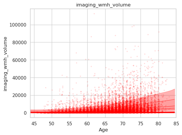
Here a simple scatterplot of the raw data.

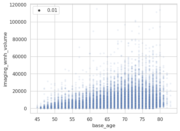
The problem is apparent when looking at other imaging-derived phenotypes.

Disconnectivity of the arcuate fascicle in percent using the abovementioned plotting code. Note that the data is shifted upwards (y interval is 20-120% instead of 0-100%).

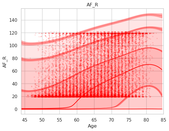
And the corresponding raw data plot.

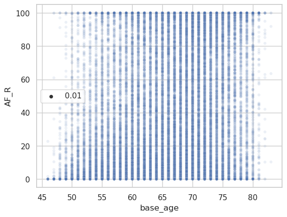
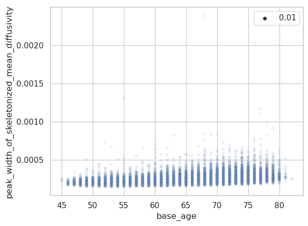
The same plots for the peak width of skeletonized mean diffusivity (PSMD).

Are there some assumptions that need to be met to apply warped BLR when modelling a variable, like is non-gaussianity of residuals required? One difference to the tutorials is that I use a 2-fold cross-validation via estimate() to get zscores for all individuals. I noticed that the resulting centile curves differ relevantly if I rerun the analysis. Maybe because of probabilistic sampling of training and test set during CV?

The complete code I use can be found in this jupyter notebook: https://drive.google.com/file/d/1p0jHzDC832yVKWd7p0PULgfhbnnYUi0F/view?usp=sharing.

I would be very grateful to get some help. Happy to provide further information if required.

Thanks a lot in advance!

Marvin

[amarquand]

Hi, there are a few things going on here. First, the only reason the data are rescaled is for visualization purposes, ie. to plot all the sites against a common set of centiles (otherwise each site will be different). If you plot each site separately it is not necessary. Also you probably do not even need to worry about site effects if you are using UKB data and a phenotype like that.

Second, it is important to understand that the warp implicitly uses a SHASH distribution which is good for continuous data and can model many shapes. But there are also a lot of distributions it cannot fit and for the interval data you show (arcuate) you will never achieve an acceptable fit. You would be better to use a beta distribution instead which is not currently supported in pcntoolkit but might be at some point. See here (and the references therein) for more details about the SHASH dist: https://www.biorxiv.org/content/10.1101/2022.10.05.510988v2

The last example is an optimization failure which you might be able to fix by changing the optimizer or regularization settings. You also should know that fitting shape parameters is a very hard optimization problem in general because of strong dependencies between parameters and often weak identifiability of different parameter values.

[amarquand]

Hi again - just to elaborate on my previous post. For the last optimization error you can try changing the optimizer to 'powell' and see if that works

[amarquand]

Hi - I would just like to follow up on this again. I just noticed that you have some very severe outliers in the plot for peak_width_of_skeletonized_mean_diffusivity. Did you quality check your data before fitting your models? points like these can have a lot of leverage on the outer centiles (which are actually the only ones not really fit well by the warp). I would not be surprised to see your fit improve considerably after doing a careful quality check of your data.

I will close this issue now, because there are some conceptual issues that need to be addressed. I don't think it is necessarily a problem with the code. Feel free to reach out (e.g. via gitter) if you would like to discuss further.

[m-petersen]

Hi Andre,

Thank you for your response and the clarifications. As I am still familiarizing myself with the theoretical aspects of normative modelling, the context you have provided has been very helpful.

Thanks for pointing out the outliers, which I should have recognized as a possible issue. Currently, the PSMD has not undergone quality assessment, as we are still discussing how to address quality assurance for UKB data in a systematic and feasible manner, given its large scale. So the plots I am showing here are just results from me exploring PCNtoolkit for the downstream analysis once the imaging data has been curated and quality checked. I will reconduct the modelling once the QA is done and also try your recommendation with regard to switching the optimizer.

I am very grateful for your time and help.

Best Marvin