Closed daybrown closed 3 years ago
Hi,
As I told you on discourse, this is a bit "border line" for my package which targets PDEs. However, I am currently improving a lot the interface so ODE can be studied too in regimes where this is really difficult for PDE (like homoclinic orbits,...). Indeed, with these improvements, you will be able to use much larger M
than before (for Shooting methods and FD ones). However, it brings another problem: my computation of the Floquet coefficients become unstable for large M
s (but I am working on it). So using detectBifurcation = 2
is likely to give spurious bifurcations for now.
I will soon announce these improvements and document them with an ODE application.
For the FD method, you can do:
# automatic branch switching from Hopf point
opt_po = NewtonPar(tol = 1e-5, verbose = true, maxIter = 15)
opts_po_cont = ContinuationPar(dsmin = 0.0001, dsmax = 0.1, ds = 0.001, pMax = 5.5, pMin=-2.1, maxSteps = 200, newtonOptions = opt_po, saveSolEveryStep = 2, plotEveryStep = 1, nev = 11, precisionStability = 1e-4, detectBifurcation = 0, dsminBisection = 1e-4, maxBisectionSteps = 10);
# number of time slices for the periodic orbit
M = 251
br_po, = continuation(
# arguments for branch switching from the first
# Hopf bifurcation point
jet..., br, 1,
# arguments for continuation
setproperties(opts_po_cont; ds = -0.001, dsmax = 0.1),
PeriodicOrbitTrapProblem(M = M);
# to find non trivial periodic orbits
usedeflation = true,
# to update the section during continuation
updateSectionEveryStep = 1,
# OPTIONAL parameters
# we want to jump on the new branch at phopf + δp
# ampfactor is a factor to increase the amplitude of the guess
δp = 0.003, ampfactor = 1.0,
# specific method for computing the Jacobian
linearPO = :Dense,
# regular options for continuation
verbosity = 3, plot = true,
printSolution = (x, p) -> begin
xtt=reshape(x[1:end-1],2,M);
return (max = maximum(xtt[1,:]), min = minimum(xtt[1,:]), period = x[end])
end,
plotSolution = (x,p; k...) -> begin
xtt = BK.getTrajectory(p.prob, x, p.p)
plot!(xtt.t, xtt.u[1,:]; label = "x", k...)
plot!(xtt.t, xtt.u[2,:]; label = "y", k...)
plot!(br, legend = false; subplot = 1)
end,
normC = norminf)
It gives:
For the Shooting method, it is very similar:
probsh = ODEProblem(Fitz!, copy(sol0), (0., 1000.), par_Fitz; atol = 1e-10, rtol = 1e-9)
br_po, = continuation(
# arguments for branch switching from the first
# Hopf bifurcation point
jet..., br, 1,
# arguments for continuation
setproperties(opts_po_cont; ds = -0.001, dsmax = 0.31, detectBifurcation = 0),
ShootingProblem(25, par_Fitz, probsh, Rodas4(), parallel = true);
usedeflation = false,
# OPTIONAL parameters
# we want to jump on the new branch at phopf + δp
# ampfactor is a factor to increase the amplitude of the guess
δp = 0.001, ampfactor = 1.0,
# specific method for computing the Jacobian
linearPO = :autodiffDense,
updateSectionEveryStep = 2,
# regular options for continuation
verbosity = 3, plot = true,
printSolution = (x, p) -> begin
(max = getMaximum(p.prob, x, @set par_Fitz.I = p.p), period = getPeriod(p.prob, x, @set par_Fitz.I = p.p))
end,
plotSolution = (x,p; k...) -> begin
xtt = BK.getTrajectory(p.prob, x, @set par_Fitz.I = p.p)
plot!(xtt; k...)
plot!(br, legend = false; subplot = 1)
end,
normC = norminf)
But it does not work that well, I think this is because of the section.
Best.
So the results are depend on those improvements? I got the following error with the code you provide:
MethodError: no method matching ContIterable(::PeriodicOrbitTrapProblem{typeof(Fitz),typeof(dFbpSecBif),Nothing,Nothing,Nothing,Array{Float64,1},DefaultLS,BifurcationKit.TimeMesh{Int64}}, ::BifurcationKit.var"#617#625"{PeriodicOrbitTrapProblem{typeof(Fitz),typeof(dFbpSecBif),Nothing,Nothing,Nothing,Array{Float64,1},DefaultLS,BifurcationKit.TimeMesh{Int64}}}, ::Array{Float64,1}, ::NamedTuple{(:I, :a, :b, :c),NTuple{4,Float64}}, ::Setfield.PropertyLens{:I}, ::ContinuationPar{Float64,BifurcationKit.POTrapLinsolver{DefaultLS},DefaultEig{typeof(real)}}, ::BorderingBLS{BifurcationKit.POTrapLinsolver{DefaultLS},Float64}; printSolution=var"#326#329"(), updateSectionEveryStep=1, verbosity=3, plot=true, plotSolution=var"#327#330"(), normC=var"#252#253"())
are you on master?
I am not sure what you mean? I am working on Jupyter notebook.
did you do ] add BifurcationKit#master
?
No.
I did that, still the same error. Should I restart the session?
Probably.
Now it works, but it gives:
And the output is:
(Branch number of points: 201 Branch of PeriodicOrbit from Hopf bifurcation point. Parameters from -0.5446740802107838 to -0.544957143775975 Fold points: , BorderedArray{Array{Float64,1},Float64}([-0.968514292075122, -1.2106428650919805, -0.9685142920767131, -1.2106428650919685, -0.9685142920782126, -1.210642865091894, -0.9685142920796487, -1.2106428650917336, -0.9685142920809898, -1.210642865091484 … -1.2106428650912708, -0.968514292069922, -1.210642865091536, -0.9685142920717401, -1.2106428650917511, -0.9685142920734605, -1.2106428650919137, -0.968514292075122, -1.2106428650919805, -581.6947989161991], -0.5449571437758539), BorderedArray{Array{Float64,1},Float64}([-2.9531932455029623e-13, -8.593126210598846e-13, -4.551914400963213e-14, -8.859579736508888e-13, 1.8318679906315368e-13, -9.281464485866454e-13, 3.9412917374193673e-13, -9.880984919164047e-13, 5.839773109528414e-13, -1.0658141036401668e-12 … -9.303668946358957e-13, -1.1590728377086816e-12, -8.881784197001392e-13, -8.504308368628832e-13, -8.615330671091349e-13, -5.639932965095883e-13, -8.504308368628832e-13, -2.9531932455029623e-13, -8.593126210598846e-13, 31.717503054307414], -1.2112533198660648e-12))
OK, I did not push the deflation of periodic orbits. You can try using a larger amplification factor (it works for me)
br_potrap, = continuation(
# arguments for branch switching from the first
# Hopf bifurcation point
jet..., br, 1,
# arguments for continuation
setproperties(opts_po_cont; ds = -0.001, dsmax = 0.1),
PeriodicOrbitTrapProblem(M = M);
# to update the section during continuation
updateSectionEveryStep = 1,
# OPTIONAL parameters
# we want to jump on the new branch at phopf + δp
# ampfactor is a factor to increase the amplitude of the guess
δp = 0.001, ampfactor = 2.0,
# # specific method for computing the Jacobian
linearPO = :Dense,
# regular options for continuation
verbosity = 3, plot = true,
printSolution = (x, p) -> begin
xtt=reshape(x[1:end-1],2,M);
return (max = maximum(xtt[1,:]), min = minimum(xtt[1,:]), period = x[end])
end,
plotSolution = (x,p; k...) -> begin
xtt = BK.getTrajectory(p.prob, x, p.p)
plot!(xtt.t, xtt.u[1,:]; label = "x", k...)
plot!(xtt.t, xtt.u[2,:]; label = "y", k...)
plot!(br, legend = false; subplot = 1)
end,
normC = norminf)
Now it works! Thank you. It's really sensitive to the parameters (like δp).
Super!
If you see the shape of the curve, it is not surprising... I think the problems of spurious fold stems from my section which is not global. I will address it.
Hi,
On master, I have the following. Note that the Floquet coefficients will need more work to be computed reliably for a large number of time sections. Should we close this issue?
opt_po = NewtonPar(tol = 1e-9, verbose = true, maxIter = 25)
opts_po_cont = ContinuationPar(dsmin = 0.0001, dsmax = 0.1, ds = 0.001, pMax = 5.5, pMin=-2.1, maxSteps = 110, newtonOptions = opt_po, saveSolEveryStep = 1, plotEveryStep = 1, nev = 11, precisionStability = 1e-4, detectBifurcation = 0, dsminBisection = 1e-4, maxBisectionSteps = 10);
# number of time slices for the periodic orbit
M = 251
br_potrap, u1 = continuation(
# arguments for branch switching from the first
# Hopf bifurcation point
jet..., br, 1,
# arguments for continuation
setproperties(opts_po_cont; ds = 0.001, dsmax = 0.1),
PeriodicOrbitTrapProblem(M = M);
# to find non trivial periodic orbits
usedeflation = true,
# to update the section during continuation
updateSectionEveryStep = 1,
# OPTIONAL parameters
# we want to jump on the new branch at phopf + δp
# ampfactor is a factor to increase the amplitude of the guess
δp = 0.001, ampfactor = 2.0,
# # specific method for computing the Jacobian
linearPO = :Dense,
# regular options for continuation
verbosity = 3, plot = true,
printSolution = (x, p) -> begin
xtt=reshape(x[1:end-1],2,M);
return (max = maximum(xtt[1,:]), min = minimum(xtt[1,:]), period = x[end])
end,
plotSolution = (x,p; k...) -> begin
xtt = BK.getTrajectory(p.prob, x, p.p)
plot!(xtt.t, xtt.u[1,:]; label = "x", k...)
plot!(xtt.t, xtt.u[2,:]; label = "y", k...)
plot!(br, legend = false; subplot = 1)
end,
finaliseSolution = (z, tau, step, contResult; k...) ->
(Base.display(contResult.eig[end].eigenvals) ;true),
normC = norminf)
Looks great! Thank you. Yes, we should close.
On Tue, Dec 1, 2020, 2:22 PM Romain Veltz notifications@github.com wrote:
Hi,
On master, I have the following. Note that the Floquet coefficients will need more work to be computed reliably for a large number of time sections. Should we close this issue?
opt_po = NewtonPar(tol = 1e-9, verbose = true, maxIter = 25)
opts_po_cont = ContinuationPar(dsmin = 0.0001, dsmax = 0.1, ds = 0.001, pMax = 5.5, pMin=-2.1, maxSteps = 110, newtonOptions = opt_po, saveSolEveryStep = 1, plotEveryStep = 1, nev = 11, precisionStability = 1e-4, detectBifurcation = 0, dsminBisection = 1e-4, maxBisectionSteps = 10);
number of time slices for the periodic orbit
M = 251
br_potrap, u1 = continuation(
arguments for branch switching from the first
Hopf bifurcation point
jet..., br, 1,
arguments for continuation
setproperties(opts_po_cont; ds = 0.001, dsmax = 0.1),
PeriodicOrbitTrapProblem(M = M);
to find non trivial periodic orbits
usedeflation = true,
to update the section during continuation
updateSectionEveryStep = 1,
OPTIONAL parameters
we want to jump on the new branch at phopf + δp
ampfactor is a factor to increase the amplitude of the guess
δp = 0.001, ampfactor = 2.0,
specific method for computing the Jacobian
linearPO = :Dense,
regular options for continuation
verbosity = 3, plot = true,
printSolution = (x, p) -> begin
xtt=reshape(x[1:end-1],2,M); return (max = maximum(xtt[1,:]), min = minimum(xtt[1,:]), period = x[end]) end,
plotSolution = (x,p; k...) -> begin
xtt = BK.getTrajectory(p.prob, x, p.p) plot!(xtt.t, xtt.u[1,:]; label = "x", k...) plot!(xtt.t, xtt.u[2,:]; label = "y", k...) plot!(br, legend = false; subplot = 1) end,
finaliseSolution = (z, tau, step, contResult; k...) ->
(Base.display(contResult.eig[end].eigenvals) ;true),
normC = norminf)
[image: Screen Shot 2020-12-01 at 20 20 56] https://user-images.githubusercontent.com/1591812/100786715-d30f8f00-3412-11eb-909b-a2ba48be423a.png
— You are receiving this because you authored the thread. Reply to this email directly, view it on GitHub https://github.com/rveltz/BifurcationKit.jl/issues/28#issuecomment-736764848, or unsubscribe https://github.com/notifications/unsubscribe-auth/AKE472FNUFFBSESU7QX6KZTSSU67LANCNFSM4TY2M4HQ .
I expect to get the following result in AUTO. Though I already have the result, I am looking for a pure Julia package to handle this kind of problem.
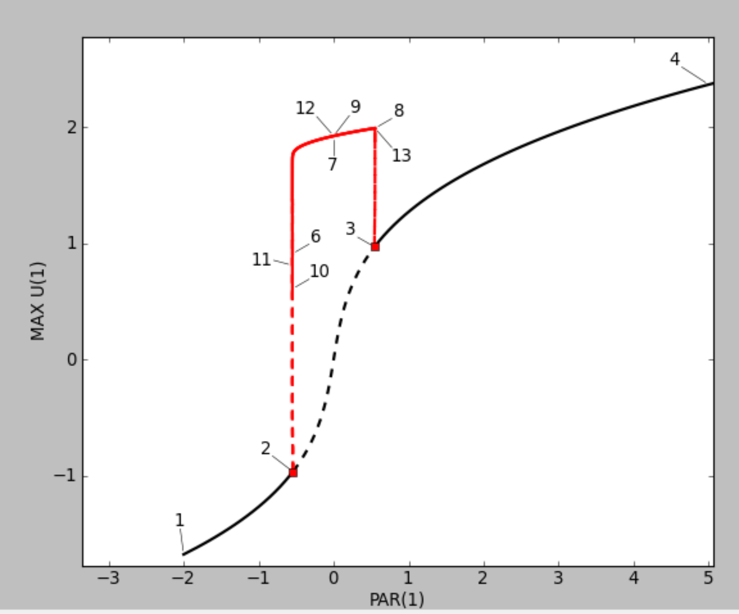
My question is how do I modify the code to get a similar result?