 mitchhitch
commented
4 years ago
mitchhitch
commented
4 years ago I have the exact same issue and this whole package is useless without this function.
Open bettyliao776 opened 4 years ago
mitchhitch
commented
4 years ago I have the exact same issue and this whole package is useless without this function.
 mdancho84
commented
4 years ago
mdancho84
commented
4 years ago Hey, I'm sorry about this. I'm transitioning most of this functionality over to timetk so you may have better luck with that. I'm not in a position to work on anomalize (my apologies). I'd try:
library(timetk)
library(tidyverse)

# Get Anomaly Data
walmart_sales_weekly %>%
    group_by(id) %>%
    tk_anomaly_diagnostics(
        .date_var = Date,
        .value    = Weekly_Sales
    )
#> frequency = 13 observations per 1 quarter
#> trend = 52 observations per 1 year
#> frequency = 13 observations per 1 quarter
#> trend = 52 observations per 1 year
#> frequency = 13 observations per 1 quarter
#> trend = 52 observations per 1 year
#> frequency = 13 observations per 1 quarter
#> trend = 52 observations per 1 year
#> frequency = 13 observations per 1 quarter
#> trend = 52 observations per 1 year
#> frequency = 13 observations per 1 quarter
#> trend = 52 observations per 1 year
#> frequency = 13 observations per 1 quarter
#> trend = 52 observations per 1 year
#> # A tibble: 1,001 x 12
#> # Groups:   id [7]
#>    id    Date       observed season  trend remainder seasadj remainder_l1
#>    <fct> <date>        <dbl>  <dbl>  <dbl>     <dbl>   <dbl>        <dbl>
#>  1 1_1   2010-02-05   24924.   874. 19967.     4083.  24050.      -15981.
#>  2 1_1   2010-02-12   46039.  -698. 19835.    26902.  46737.      -15981.
#>  3 1_1   2010-02-19   41596. -1216. 19703.    23108.  42812.      -15981.
#>  4 1_1   2010-02-26   19404.  -821. 19571.      653.  20224.      -15981.
#>  5 1_1   2010-03-05   21828.   324. 19439.     2064.  21504.      -15981.
#>  6 1_1   2010-03-12   21043.   471. 19307.     1265.  20572.      -15981.
#>  7 1_1   2010-03-19   22137.   920. 19175.     2041.  21217.      -15981.
#>  8 1_1   2010-03-26   26229.   752. 19069.     6409.  25478.      -15981.
#>  9 1_1   2010-04-02   57258.   503. 18962.    37794.  56755.      -15981.
#> 10 1_1   2010-04-09   42961.  1132. 18855.    22974.  41829.      -15981.
#> # … with 991 more rows, and 4 more variables: remainder_l2 <dbl>,
#> #   anomaly <chr>, recomposed_l1 <dbl>, recomposed_l2 <dbl>

# Plot Anomalies
walmart_sales_weekly %>%
    group_by(id) %>%
    plot_anomaly_diagnostics(
        .date_var    = Date,
        .value       = Weekly_Sales,
        .facet_ncol  = 2,
        .interactive = FALSE
    )
#> frequency = 13 observations per 1 quarter
#> trend = 52 observations per 1 year
#> frequency = 13 observations per 1 quarter
#> trend = 52 observations per 1 year
#> frequency = 13 observations per 1 quarter
#> trend = 52 observations per 1 year
#> frequency = 13 observations per 1 quarter
#> trend = 52 observations per 1 year
#> frequency = 13 observations per 1 quarter
#> trend = 52 observations per 1 year
#> frequency = 13 observations per 1 quarter
#> trend = 52 observations per 1 year
#> frequency = 13 observations per 1 quarter
#> trend = 52 observations per 1 year
Created on 2020-11-13 by the reprex package (v0.3.0)
Hi, I run the sample code from https://github.com/business-science/anomalize and there's an issue. Please see below: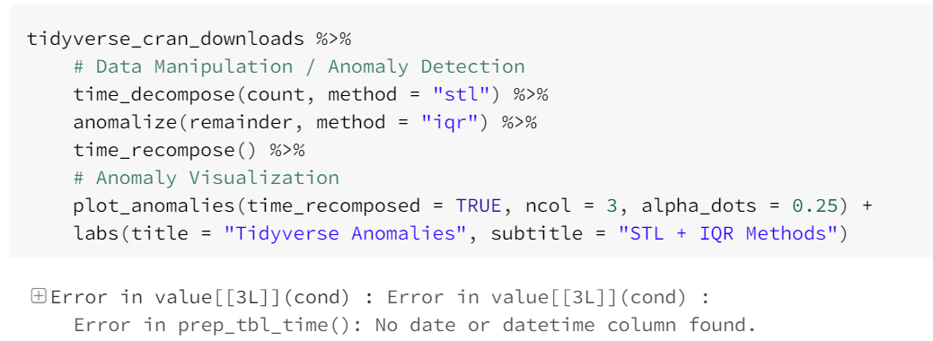
I tried the same code on my own tibble table and I got the same error: Error in value[3L] : Error in value[3L] : Error in prep_tbl_time(): No date or datetime column found.