[Bug] Posterior variance big compare to GPy for large N

[tmpethick]

🐛 Bug

I am trying to fit f(x) = sin(60 x⁴) with a gpytorch.kernels.ScaleKernel(gpytorch.kernels.RBFKernel()) kernel with many observations (N=1000). I have fixed the hyperparameters but the posterior variance seems to be much bigger than for GPy (see plots further down). We would expect it to approach zero everywhere for this many observations. Do you have a clue from where the instability could come?

To reproduce

Code snippet to reproduce

import math
import numpy as np
import torch
import gpytorch
from matplotlib import pyplot as plt

def gpytorch_model(noise=0.5, lengthscale=2.5, variance=2, n_iter=200):
    bounds = np.array([[0,1]])
    train_x = torch.linspace(bounds[0,0], bounds[0,1], 999).double()
    train_y = np.sin(60 * train_x ** 4)

    class ExactGPModel(gpytorch.models.ExactGP):
        def __init__(self, train_x, train_y, likelihood):
            super(ExactGPModel, self).__init__(train_x, train_y, likelihood)
            self.mean_module = gpytorch.means.ZeroMean()
            self.covar_module = gpytorch.kernels.ScaleKernel(
                gpytorch.kernels.RBFKernel())

        def forward(self, x):
            mean_x = self.mean_module(x)
            covar_x = self.covar_module(x)
            return gpytorch.distributions.MultivariateNormal(mean_x, covar_x)

    # initialize likelihood and model
    likelihood = gpytorch.likelihoods.GaussianLikelihood()
    model = ExactGPModel(train_x, train_y, likelihood)
    model = model.double()

    model.initialize(**{
        'likelihood.noise': noise,
        'covar_module.base_kernel.lengthscale': lengthscale,
        'covar_module.outputscale': variance,
    })
    print("lengthscale: %.3f, variance: %.3f,   noise: %.5f" % (model.covar_module.base_kernel.lengthscale.item(),
            model.covar_module.outputscale.item(),
            model.likelihood.noise.item()))

    # Find optimal model hyperparameters
    model.train()
    likelihood.train()

    # Use the adam optimizer
    optimizer = torch.optim.Adam([
        {'params': model.parameters()}, 
    ], lr=0.1)

    # "Loss" for GPs - the marginal log likelihood
    mll = gpytorch.mlls.ExactMarginalLogLikelihood(likelihood, model)

    for i in range(n_iter):
        # Zero gradients from previous iteration
        optimizer.zero_grad()
        # Output from model
        output = model(train_x)
        # Calc loss and backprop gradients
        loss = -mll(output, train_y)
        loss.backward()

        optimizer.step()

    # Prediction
    # Get into evaluation (predictive posterior) mode
    model.eval()
    likelihood.eval()

    # Test points are regularly spaced along [0,1]
    # Make predictions by feeding model through likelihood
    with torch.no_grad():
        test_x = torch.linspace(bounds[0,0], bounds[0,1], 1000).double()
        observed_pred = likelihood(model(test_x))

        # Initialize plot
        f, ax = plt.subplots(1, 1, figsize=(8, 3))

        # Get upper and lower confidence bounds
        var = observed_pred.variance.numpy()
        mean = observed_pred.mean.numpy()
        lower, upper = mean - 2 * np.sqrt(var), mean + 2 * np.sqrt(var)
        # Plot training data as black stars
        ax.plot(train_x.numpy(), train_y.numpy(), 'k*')
        # Plot predictive means as blue line
        ax.plot(test_x.numpy(), mean, 'b')
        # Shade between the lower and upper confidence bounds
        ax.fill_between(test_x.numpy(), lower, upper, alpha=0.5)
        ax.legend(['Observed Data', 'Mean', 'Confidence'])
    return model, {
        'lengthscale': model.covar_module.base_kernel.lengthscale.item(),
        'variance': model.covar_module.outputscale.item(),
        'noise': model.likelihood.noise.item(),
    }

model, params = gpytorch_model(noise=0.0001, lengthscale=0.015, variance=9, n_iter=0)

Stack trace/error message

Expected Behavior

We expect similar behaviour to GPy:

But got:

System information

GPyTorch Version: 0.3.2 PyTorch Version: 1.0.1.post2 Computer OS: MacOS 10.14

Additional context

Code to reproduce the GPy plot:

import math
import torch
import numpy as np
from matplotlib import pyplot as plt
import GPy

def gpy_model(noise=0.5, lengthscale=2.5, variance=2, optimize=True):
    def f(x):
        x = np.asanyarray(x)
        y = where(x == 0, 1.0e-20, x)
        return np.sin(y)/y

    bounds = np.array([[0,1]])
    train_x = torch.linspace(bounds[0,0], bounds[0,1], 999)
    train_y = np.sin(60 * train_x ** 4)

    kernel = GPy.kern.RBF(1, ARD=False)
    model = GPy.models.GPRegression(train_x.numpy()[:,None], train_y.numpy()[:,None], kernel=kernel)
    model.Gaussian_noise = noise
    model.kern.lengthscale = lengthscale
    model.kern.variance = variance

    if optimize:
        model.optimize()

    test_x = np.linspace(bounds[0,0], bounds[0,1], 1000)
    mean, var = model.predict(test_x[:, None])
    mean = mean[:,0]
    var = var[:,0]

    # Initialize plot
    f, ax = plt.subplots(1, 1, figsize=(8, 3))

    # Get upper and lower confidence bounds
    lower, upper = mean - 2 * np.sqrt(var), mean + 2 * np.sqrt(var)
    # Plot training data as black stars
    ax.plot(train_x.numpy(), train_y.numpy(), 'k*')
    # Plot predictive means as blue line
    ax.plot(test_x, mean, 'b')
    # Shade between the lower and upper confidence bounds
    ax.fill_between(test_x, lower, upper, alpha=0.5)
    ax.legend(['Observed Data', 'Mean', 'Confidence'])

    #print("l: {}, v: {}, noise: {}".format(kernel.lengthscale, kernel.variance, model.Gaussian_noise.variance))
    return model, {
        'lengthscale': kernel.lengthscale,
        'noise': model.Gaussian_noise.variance,
        'variance': kernel.variance
    }

model, params = gpy_model(noise=0.0001, lengthscale=0.015, variance=9, optimize=False)

[tmpethick]

This seems to happen because GPyTorch defaults to fast computations. We recover the correct posterior if we disable preconditioned CG by wrapping the posterior in the following:

with gpytorch.settings.fast_computations(covar_root_decomposition=True, log_prob=True, solves=False):
    # posterior calc...

Interestingly enough the exact version is much faster in this case... (I am guessing CG is only really useful when N becomes truly big). Maybe these (default) "approximations" should be made more explicit if they can lead to weird behaviour?

PS: As far as I remember CG should actually give an exact solution provided enough steps. I will look into whether we can configurate it differently to reproduce the exact posterior...

[tmpethick]

Following https://github.com/cornellius-gp/gpytorch/issues/377 I tried increasing every possible knob:

with gpytorch.settings.max_lanczos_quadrature_iterations(32),\
        gpytorch.settings.fast_computations(covar_root_decomposition=False, log_prob=False, solves=True), \
        gpytorch.settings.max_cg_iterations(2000), \
        gpytorch.settings.max_preconditioner_size(20),\
        gpytorch.settings.num_trace_samples(128):
    # predict

However, we still get too high variance even for a simple sin (when N=1000):

Compare to the following where cholesky is used (i.e. gpytorch.settings.fast_computations(solves=False)):

In general this happens when the noise level is too low (e.g. noise=0.0001). Then the posterior which CG converges to is similar to a model with noise=0.01 except the variance is less smooth.

It seems weird that we can't converge even when putting practically no restriction on number of iterations, samples etc.. Any ideas?

---

Code to reproduce CG plot (note that even if we add a significant amount of noise with train_y = train_y + 0.2 * torch.randn_like(train_y) the problem still persists):

import math
import numpy as np
import torch
import gpytorch
from matplotlib import pyplot as plt
def gpytorch_model(noise=0.5, lengthscale=2.5, variance=2, n_iter=200):
    bounds = np.array([[0,1]])
    train_x = torch.linspace(bounds[0,0], bounds[0,1], 999).double()
    train_y = np.sin(60 * train_x ** 4)
    train_y = np.sin(100 * train_x)

    class ExactGPModel(gpytorch.models.ExactGP):
        def __init__(self, train_x, train_y, likelihood):
            super(ExactGPModel, self).__init__(train_x, train_y, likelihood)
            self.mean_module = gpytorch.means.ZeroMean()
            self.covar_module = gpytorch.kernels.ScaleKernel(gpytorch.kernels.RBFKernel())

        def forward(self, x):
            mean_x = self.mean_module(x)
            covar_x = self.covar_module(x)
            return gpytorch.distributions.MultivariateNormal(mean_x, covar_x)

    # initialize likelihood and model
    likelihood = gpytorch.likelihoods.GaussianLikelihood()
    # likelihood = gpytorch.likelihoods.FixedNoiseGaussianLikelihood(noise=torch.ones(1) * 0.0001)
    model = ExactGPModel(train_x, train_y, likelihood)
    model = model.double()

    model.initialize(**{
        'likelihood.noise': noise,
        'covar_module.base_kernel.lengthscale': lengthscale,
        'covar_module.outputscale': variance,
    })
    print("lengthscale: %.3f, variance: %.3f,   noise: %.5f" % (model.covar_module.base_kernel.lengthscale.item(),
            model.covar_module.outputscale.item(),
            model.likelihood.noise.item()))

    # Find optimal model hyperparameters
    model.train()
    likelihood.train()

    # Use the adam optimizer
    optimizer = torch.optim.Adam([
        {'params': model.parameters()}, 
    ], lr=0.1)

    # "Loss" for GPs - the marginal log likelihood
    mll = gpytorch.mlls.ExactMarginalLogLikelihood(likelihood, model)

    for i in range(n_iter):
        # Zero gradients from previous iteration
        optimizer.zero_grad()
        # Output from model
        output = model(train_x)
        # Calc loss and backprop gradients
        loss = -mll(output, train_y)
        loss.backward()

        optimizer.step()

    # Prediction
    # Get into evaluation (predictive posterior) mode
    model.eval()
    likelihood.eval()

    # Test points are regularly spaced along [0,1]
    # Make predictions by feeding model through likelihood
    with torch.no_grad(), \
        gpytorch.settings.max_lanczos_quadrature_iterations(32),\
        gpytorch.settings.fast_computations(covar_root_decomposition=False, log_prob=False, solves=True), \
        gpytorch.settings.max_cg_iterations(2000), \
        gpytorch.settings.max_preconditioner_size(20),\
        gpytorch.settings.num_trace_samples(128):

        test_x = torch.linspace(bounds[0,0], bounds[0,1], 1000).double()
        observed_pred = likelihood(model(test_x))

        # Initialize plot
        f, ax = plt.subplots(1, 1, figsize=(8, 3))

        # Get upper and lower confidence bounds
        var = observed_pred.variance.numpy()
        mean = observed_pred.mean.numpy()
        lower, upper = mean - 2 * np.sqrt(var), mean + 2 * np.sqrt(var)
        # Plot training data as black stars
        ax.plot(train_x.numpy(), train_y.numpy(), 'k*')
        # Plot predictive means as blue line
        ax.plot(test_x.numpy(), mean, 'b')
        # Shade between the lower and upper confidence bounds
        ax.fill_between(test_x.numpy(), lower, upper, alpha=0.5)
        ax.legend(['Observed Data', 'Mean', 'Confidence'])
    return model, {
        'lengthscale': model.covar_module.base_kernel.lengthscale.item(),
        'variance': model.covar_module.outputscale.item(),
        'noise': model.likelihood.noise.item(),
    }

model, params = gpytorch_model(noise=0.0001, lengthscale=0.015, variance=9, n_iter=0)

[tmpethick]

Of all the gpytorch settings the only one that seemed to effect this run in any significant way is max_preconditioner_size. Increasing it to size=80 gives the right posterior:

    with torch.no_grad(), \
        gpytorch.settings.fast_computations(covar_root_decomposition=False, log_prob=False, solves=True), \
        gpytorch.settings.max_cg_iterations(100), \
        gpytorch.settings.max_preconditioner_size(80):

Against size=70:

    with torch.no_grad(), \
        gpytorch.settings.fast_computations(covar_root_decomposition=False, log_prob=False, solves=True), \
        gpytorch.settings.max_cg_iterations(100), \
        gpytorch.settings.max_preconditioner_size(70):

This seems to require a surprisingly big preconditioner for such a simple problem...

[jacobrgardner]

A few things:

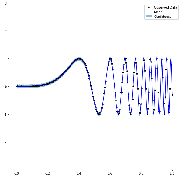
1. In the extremely low noise, I've generally found turning fast predictive variances on to be much more stable than doing the full K_{XX}^{-1}K_{XX*} solves for the predictive variances. In your case, adding gpytorch.settings.fast_pred_var() to the prediction context results in:

The reason this works better is because in the very low noise setting you have extremely small eigenvalues that would be hard to get sufficient numerical accuracy for even in double precision; fast pred var runs until a low rank approximation to K_{XX}+\sigma^{2}I is sufficiently accurate, which effectively zeros out these eigenvalues.

To answer your question in #727, turning on fast predictive variances also generally solved the issue with using fp32 as well (see below).

2. To answer your question about speed, in general, CG won't be faster than Cholesky except (a) on a GPU (where you would already see substantial speed ups over Cholesky at n=1000), or (b) in very large data regimes where Cholesky simply cannot run due to the additional O(n^2) memory cost to store L (see e.g. the multi GPU / kernel checkpointing example notebook).

3. Of all the knobs available, for extremely numerically challenging problems, increasing the preconditioner size is indeed most likely to be successful. The convergence rate of CG improves exponentially for 1D RBF problems with the size of the preconditioner (Theorem 1 of the NeurIPS paper)

fp32 Code

import math
import torch
import gpytorch
import numpy as np
from matplotlib import pyplot as plt
%matplotlib inline

bounds = np.array([[0,1]])
train_x = torch.linspace(bounds[0,0], bounds[0,1], 200)
train_y = np.sin(60 * train_x ** 4)
# We will use the simplest form of GP model, exact inference
class ExactGPModel(gpytorch.models.ExactGP):
    def __init__(self, train_x, train_y, likelihood):
        super(ExactGPModel, self).__init__(train_x, train_y, likelihood)
        self.mean_module = gpytorch.means.ZeroMean()
        self.covar_module = gpytorch.kernels.ScaleKernel(gpytorch.kernels.MaternKernel())

    def forward(self, x):
        mean_x = self.mean_module(x)
        covar_x = self.covar_module(x)
        return gpytorch.distributions.MultivariateNormal(mean_x, covar_x)

# initialize likelihood and model
likelihood = gpytorch.likelihoods.GaussianLikelihood()
model = ExactGPModel(train_x, train_y, likelihood)

print("Initialized with: lengthscale=%.3f variance=%.3f noise=%.5f" % (model.covar_module.base_kernel.lengthscale.item(),
        model.covar_module.outputscale.item(),
        model.likelihood.noise.item()))

# Find optimal model hyperparameters
model.train()
likelihood.train()

# Use the adam optimizer
optimizer = torch.optim.Adam([
    {'params': model.parameters()}, 
], lr=0.1)

# "Loss" for GPs - the marginal log likelihood
mll = gpytorch.mlls.ExactMarginalLogLikelihood(likelihood, model)

training_iter = 150
for i in range(training_iter):
    # Zero gradients from previous iteration
    optimizer.zero_grad()
    # Output from model
    output = model(train_x)
    # Calc loss and backprop gradients
    loss = -mll(output, train_y)
    loss.backward()
    print('Iter %d/%d - Loss: %.3f   lengthscale: %.3f, variance: %.3f,   noise: %.5f' % (
        i + 1, training_iter, loss.item(),
        model.covar_module.base_kernel.lengthscale.item(),
        model.covar_module.outputscale.item(),
        model.likelihood.noise.item()
    ))
    optimizer.step()

# Prediction
# Get into evaluation (predictive posterior) mode
model.eval()
likelihood.eval()

# Test points are regularly spaced along [0,1]
# Make predictions by feeding model through likelihood
with torch.no_grad(), gpytorch.settings.fast_pred_var():
    test_x = torch.linspace(bounds[0,0], bounds[0,1], 1000)
    observed_pred = likelihood(model(test_x))

    # Initialize plot
    f, ax = plt.subplots(1, 1, figsize=(10, 10))

    # Get upper and lower confidence bounds
    lower, upper = observed_pred.confidence_region()
    # Plot training data as black stars
    ax.plot(train_x.numpy(), train_y.numpy(), 'k*')
    # Plot predictive means as blue line
    ax.plot(test_x.numpy(), observed_pred.mean.numpy(), 'b')
    # Shade between the lower and upper confidence bounds
    ax.fill_between(test_x.numpy(), lower.numpy(), upper.numpy(), alpha=0.5)
    ax.set_ylim([-3, 3])
    ax.legend(['Observed Data', 'Mean', 'Confidence'])

Produces:

[jacobrgardner]

Sorry, one other question you asked I forgot to answer: in general it's quite straight forward to detect when you are having numerical problems (you asked about when to add noise). GPyTorch spits out a warning as you noticed when CG is failing to converge.

In general, no warning means CG was giving you exact GP results, and a warning usually means there was trouble, and you will want to e.g. expend more compute on the solves.

[tmpethick]

I am happily surprised every time by the amount of effort you put into your replies - thanks! Fast predictive variance does the trick – I will have to read into it.

It seems very interesting that an approximation that is asymptotically faster can lead to better performance. Is there any paper pointing out/elaborating on this potential benefit for low noise settings?

[jacobrgardner]

Yeah, so it's a good question. I would conjecture that for something like the pivoted Cholesky decomposition or Lanczos, we could indeed prove exponential convergence in ||K - L_kL_k'||, where L_k is the decomposition (either from pivoted Cholesky, or by computing QT^{1/2} from Lanczos).

In our paper, we observe at least empirically that, for example, CG can sometimes provide better solve residuals than Cholesky in fp32 (see Figure 2). This occurs for the same "regularizing" effect.

I think it is well known that this can occasionally happen in the scientific computing literature. I've asked @dme65 -- we'll see if we can dig up a reference for this phenomenon.