Closed tvanbutselaar closed 5 years ago
Hi Tijmen @tvanbutselaar ,
I can certainly look into it! I have also seen it where small leaves get clustered differently and it can be hard to see which color they are labeled when they are so small. We added the show_grid
parameter to pcv.cluster_contours
to assist with this. I think that labeling could be useful so I'll plan to play around with a feature like this.
Would you mind sending an example image that is difficult to decluster and the workflow you are using?
Dear Haley, Sorry for the tardy response. I have attached an example image from a set of around 20 pictures that I found was difficult to decluster. One issue in this image is the touching of some plant parts, which is something that I will tackle in new pictures as I do not think can be solved here that easily.
Thanks
The wrapper shell script I use to analyze the set of pictures is:
#!/bin/bash
#Execute script with cwd as directory where your input folder with images is (by default this should be a directory on virtualbox shared folder, to prevent the ubuntu drive from clogging up). Execute the script as follows: bash plantcvbash.sh [name of input folder in pwd] [name of output folder in pwd]
#Main description and warnings
mpwd=$(pwd)
mkdir ~/PlantCV
mkdir ~/PlantCV/tmp
mkdir $mpwd/$2
#Set up the main variable list. These parameters will be called on in the image analysis pipelineThese are the primary parameters that need to be adjusted for your images. Take especially care that images taken by another camera than Hans' will have different sizes, therefor ROI and fill size need to be adjusted.
cat <<\EOF > $mpwd/$2/variables.txt
0 ## Script 1+2 ROI x_adj the top-left pixel defining the rectangle of ROI
0 ## Script 1+2 ROI y_adj the top-left pixel defining the rectangle of ROI
4100 ## Script 1+2 ROI w_adj value for how far along y-axis from top-left pixel the ROI stretches
6600 ## Script 1+2 ROI h_adj value for how far along x-axis from top-left pixel the ROI stretches
6 ## Script 1 cluster nrow value for number of rows of cluster. if plants parts are identified okay, but are not declustered correctly, this is the main parameter to tweak
9 ## Script 1 cluster ncol value for number of columns to cluster. if plants parts are identified okay, but are not declustered correctly, this is the main parameter to tweak
0.5 ## Script 1 rotation_deg rotation angle in degrees, can be a negative number, positive values move counter clockwise
350 ## Script 1 shift number value for shifting image up x pixels, must be greater than 1
150 ## Script 1 shift number value for shifting image left x pixels, must be greater than 1
120 ## Script 1 bin treshold threshold value (0-255) for binary tresholding, higher values will generate more background. if missing a lot of plant parts, or you have too much background, this is the main parameter to tweak
3000 ## Script 1 fill size minimum pixel size for objects, those smaller will be filled
1 ## Script 1 dilation kernel an odd integer that is used to build a ksize x ksize matrix using np.ones. Must be greater than 1 to have an effect. Greater values will ensure all plant parts are included, but also will overestimate size of plant
1 ## Script 1 dilation iter number of consecutive filtering passes for dilation. Greater values will ensure all plant parts are included, but also will overestimate size of plant
EOF
#Generate main python script for declustering pictures
cat <<\EOF > $mpwd/$2/python1.py
#!/usr/bin/python
import warnings
warnings.simplefilter(action='ignore', category=FutureWarning)
import sys, traceback
import os
import re
import numpy as np
import argparse
import string
import glob
import shutil
from PIL import Image
from plantcv import plantcv as pcv
### Parse command-line arguments
def options():
parser = argparse.ArgumentParser(description="Imaging processing with opencv")
parser.add_argument("-i", "--input", help="Input image directory.", required=True)
parser.add_argument("-o", "--outdir", help="Output directory for image files.", required=True)
parser.add_argument("-n", "--names", help="path to txt file with names of genotypes to split images into", required =False)
parser.add_argument("-r","--result", help="result file.", required= False )
parser.add_argument("-D", "--debug", help="Turn on debug, prints intermediate images.", action=None)
parser.add_argument("-v", "--variables",help="List of variables to be passed to pipeline", required=True)
args = parser.parse_args()
return args
def main(img8,tray, args, pwd):
# Get options
args = options()
if args.names!= None:
args.names="../../names/%s.txt" %(str(tray))
print("Names file: %s" %(args.names))
else:
print("No names file submitted for %s" %(str(tray)))
#Get variables from variable arguments
with open(args.variables) as f:
roi1=[line.split(' ')[0] for line in f]
# Read image
img, path, filename = pcv.readimage(img8)
pcv.params.debug=args.debug #set debug mode
# STEP 1: Check if this is a night image, for some of these dataset"s images were captured
# at night, even if nothing is visible. To make sure that images are not taken at
# night we check that the image isn"t mostly dark (0=black, 255=white).
# if it is a night image it throws a fatal error and stops the pipeline.
#if np.average(img) < 50:
# pcv.fatal_error("Night Image")
#else:
# pass
# STEP 2: Normalize the white color so you can later
# compare color between images.
# Inputs:
# img = image object, RGB colorspace
# roi = region for white reference, if none uses the whole image,
# otherwise (x position, y position, box width, box height)
# white balance image based on white toughspot
img1 = pcv.white_balance(img,roi=None)
# STEP 3: Rotate the image
rotate_img = pcv.rotate(img1, float(roi1[6]), True)
# STEP 4: Shift image. This step is important for clustering later on.
# For this image it also allows you to push the green raspberry pi camera
# out of the image. This step might not be necessary for all images.
# The resulting image is the same size as the original.
# Inputs:
# img = image object
# number = integer, number of pixels to move image
# side = direction to move from "top", "bottom", "right","left"
shift1 = pcv.shift_img(rotate_img, int(roi1[7]), "bottom")
shift2 = pcv.shift_img(shift1, int(roi1[8]), "right")
img1 = shift2
# STEP 5: Convert image from RGB colorspace to LAB colorspace
# Keep only the green-magenta channel (grayscale)
# Inputs:
# img = image object, RGB colorspace
# channel = color subchannel ("l" = lightness, "a" = green-magenta , "b" = blue-yellow)
a = pcv.rgb2gray_lab(img1, "a")
# STEP 6: Set a binary threshold on the saturation channel image
# Inputs:
# img = img object, grayscale
# threshold = threshold value (0-255)
# maxValue = value to apply above threshold (usually 255 = white)
# object_type = light or dark
# - If object is light then standard thresholding is done
# - If object is dark then inverse thresholding is done
img_binary = pcv.threshold.binary(a, int(roi1[9]), 255, "dark")
# ^
# |
# adjust this value
# STEP 7: Fill in small objects (speckles)
# Inputs:
# img = image object, grayscale. img will be returned after filling
# size = minimum object area size in pixels (integer)
fill_image = pcv.fill(img_binary, int(roi1[10]))
# ^
# |
# adjust this value
# STEP 8: Dilate so that you don"t lose leaves (just in case)
# Inputs:
# img = input image
# kernel = integer
# i = interations, i.e. number of consecutive filtering passes
dilated = pcv.dilate(fill_image, int(roi1[11]), int(roi1[12]))
# # STEP 9: Find objects (contours: black-white boundaries)
# # Inputs:
# # img = image that the objects will be overlayed
# # mask = what is used for object detection
id_objects, obj_hierarchy = pcv.find_objects(img1, dilated)
# # STEP 10: Define region of interest (ROI)
# # Inputs:
# # x_adj = adjust center along x axis
# # y_adj = adjust center along y axis
# # w_adj = adjust width
# # h_adj = adjust height
# # img = img to overlay roi
# # roi_contour, roi_hierarchy = pcv.roi.rectangle(img1, 10, 500, -10, -100)
# # ^ ^
# # |________________|
# # adjust these four values
roi_contour, roi_hierarchy = pcv.roi.rectangle(img1, int(roi1[0]), int(roi1[1]), int(roi1[2]), int(roi1[3]))
# # STEP 11: Keep objects that overlap with the ROI
# # Inputs:
# # img = img to display kept objects
# # roi_type = "cutto" or "partial" (for partially inside)
# # roi_contour = contour of roi, output from "View and Ajust ROI" function
# # roi_hierarchy = contour of roi, output from "View and Ajust ROI" function
# # object_contour = contours of objects, output from "Identifying Objects" fuction
# # obj_hierarchy = hierarchy of objects, output from "Identifying Objects" fuction
roi_objects, roi_obj_hierarchy, kept_mask, obj_area = pcv.roi_objects(img1, "partial", roi_contour, roi_hierarchy,
id_objects, obj_hierarchy)
args.debug="print"
# # STEP 12: This function take a image with multiple contours and
# # clusters them based on user input of rows and columns
# # Inputs:
# # img = An RGB image
# # roi_objects = object contours in an image that are needed to be clustered.
# # roi_obj_hierarchy = object hierarchy
# # nrow = number of rows to cluster (this should be the approximate number of desired rows in the entire image even if there isn"t a literal row of plants)
# # ncol = number of columns to cluster (thi s should be the approximate number of desired columns in the entire image even if there isn"t a literal row of plants)
# # show_grid = if True then a grid gets displayed in debug mode (default show_grid=False)
clusters_i, contours, hierarchies = pcv.cluster_contours(img1, roi_objects, roi_obj_hierarchy, int(roi1[4]), int(roi1[5]), show_grid=True)
# STEP 13: This function takes clustered contours and splits them into multiple images,
# also does a check to make sure that the number of inputted filenames matches the number
# of clustered contours. If no filenames are given then the objects are just numbered
# Inputs:
# img = ideally a masked RGB image.
# grouped_contour_indexes = output of cluster_contours, indexes of clusters of contours
# contours = contours to cluster, output of cluster_contours
# hierarchy = object hierarchy
# outdir = directory for output images
# file = the name of the input image to use as a base name , output of filename from read_image function
# filenames = input txt file with list of filenames in order from top to bottom left to right (likely list of genotypes)
# Set global debug behavior to None (default), "print" (to file), or "plot" (Jupyter Notebooks or X11)
#pcv.params.debug = "print"
out = "./"
names = args.names
output_path = pcv.cluster_contour_splitimg(img1, clusters_i, contours, hierarchies, out, file=filename, filenames=names)
args=options()
pcwd=os.getcwd()
ima=args.input
imb=ima.rsplit("/",1)[-1]
picname=ima.rsplit("/",1)[-1][:-4]
main(ima, picname, args, pcwd)
EOF
#Generate second python script for output image measurements
cat <<\EOF > $mpwd/$2/python2.py
#!/usr/bin/python
import warnings
warnings.simplefilter(action='ignore', category=FutureWarning)
import sys, traceback
import os
import re
import numpy as np
import argparse
import string
import glob
import shutil
import matplotlib
import tracemalloc as mem
from PIL import Image
from plantcv import plantcv as pcv
### Parse command-line arguments
def options():
parser = argparse.ArgumentParser(description="Imaging processing with opencv")
parser.add_argument("-i", "--input", help="Input image directory.", required=True)
parser.add_argument("-o", "--outdir", help="Output directory for image files.", required=False)
parser.add_argument("-n", "--names", help="path to txt file with names of genotypes to split images into", required =False)
parser.add_argument("-r","--result", help="result file.", required= True )
parser.add_argument("-D", "--debug", help="Turn on debug, prints intermediate images.", action=None)
parser.add_argument("-v", "--variables",help="List of variables to be passed to pipeline", required=True)
args = parser.parse_args()
return args
def analysis(image1, binary1, plantnr, tray):
args = options()
#Get variable info from variables arguments
with open(args.variables) as f:
roi1=[line.split(' ')[0] for line in f]
# Convert images to np arrays for analysis, something I have added
binarpic=Image.open(binary1)
imagpic=Image.open(image1)
binar=np.array(binarpic)
ima=np.array(imagpic)
# Find objects again within ROI, see also in main function!, from PlantCV
id_objects, obj_hierarchy = pcv.find_objects(ima, binar)
roi_contour, roi_hierarchy = pcv.roi.rectangle(ima, int(roi1[0]), int(roi1[1]), int(roi1[2]), int(roi1[3]))
#From image inputs, generate np arrays and calculate shape area, generate error if analyze_object could fail due to vertices errors, from PlantCV
roi_objects, hierarchy3, kept_mask, obj_area = pcv.roi_objects(ima, "partial", roi_contour, roi_hierarchy, id_objects, obj_hierarchy)
obj, mask = pcv.object_composition(ima, roi_objects, hierarchy3)
try:
shape_header, shape_data, shape_imgs = pcv.analyze_object(ima, obj, mask)
data=' '.join((tray, str(plantnr), str(shape_data[1])))
out=open(args.result, "a+")
out.write((data + '\n'))
out.close
except:
print("%s has not enough vertices, omitting from data.." %(str(image1)))
data=' '.join((tray,str(plantnr),"vertix_err"))
out=open(args.result, "a+")
out.write((data + '\n'))
out.close
args=options()
imga=args.input
imgb=imga[:-9] + ".jpg"
picname=imga.rsplit('/')[-1].rsplit('_')[-3]
trayname=imga.rsplit('/')[-2]
analysis(imgb, imga, picname, trayname)
EOF
#Script
for file in $mpwd/$1/* #Call all files that are in the specified input folder
do
echo "Declustering image " $file #A shout-out to stdout what image it's currently working on, so you have an idea where in your set-up it is.
picname=$(basename "$file")
picname="${picname%.*}"
mkdir ~/PlantCV/tmp/$picname #Generate temporary working directory on main drive (in stead of virtualbox shared drive, where the pictures and output will be stored mainly)
cd ~/PlantCV/tmp/$picname
python3 $mpwd/$2/python1.py -i $file -o ~/PlantCV/tmp/$picname -D print -v $mpwd/$2/variables.txt #Start the declustering of multi-plant pictures. The -D argument will ensure that also intermediary pictures of each processing step are saved. It is important to inspect these intermediary pictures after the pipeline is finished to get an idea of how the declustering behaved, and if parameters need tweaking.
for file2 in ~/PlantCV/tmp/$picname/*_mask.jpg #Call all declustered output image files
do
python3 $mpwd/$2/python2.py -i $file2 -D print -r $mpwd/$2/$picname.results.txt -v $mpwd/$2/variables.txt #Now analyze every single (supposed) plant from the declustered output
done
mv ~/PlantCV/tmp/$picname $mpwd/$2 #Move all files from the tmp folder back to the virtual shared drive, to clean up space in the virtual environment
done
cat $mpwd/$2/*.results.txt | sort > $mpwd/$2.totalresults.txt #concatenate all single image result files into one major results file. In this results file, each line is one plant (or object) with the original picture name, the plant name, and the size in squared pixels
rm -r ~/PlantCV #final cleanup
Hello @tvanbutselaar ,
Thanks for posting your workflow! We don't yet have any methods within pcv.cluster_contours
to handle different plants touching. Some data can still be collected although it will be somewhat inaccurate. For the first two plants in the 3rd column are touching, and get output as a single mask with pcv.cluster_contour_splitimg
. My suggestion to salvage these plants would be to use two circular ROI's with pcv. roi_objects
where roi_type='cutto
to create single plant masks.
I have yet to experiment with the labeling feature. However, I have gotten the example image you posted to (mostly) cooperate. The method that seemed to help was using pcv.auto_crop
, in addition to the image shifting, so that the grid better fits the plant layout. The only other change I made was increasing roi1[7]
from 350 to 450. Another potential tool that might be helpful for your other images is pcv.roi.multi
since it allows for more flexibility in layout. Below is the modifications I made to your workflow to produce the image result.
#Execute script with cwd as directory where your input folder with images is (by default this should be a directory on virtualbox shared folder, to prevent the ubuntu drive from clogging up). Execute the script as follows: bash plantcvbash.sh [name of input folder in pwd] [name of output folder in pwd]
#Main description and warnings
mpwd=$(pwd)
mkdir ~/PlantCV
mkdir ~/PlantCV/tmp
mkdir $mpwd/$2
#Set up the main variable list. These parameters will be called on in the image analysis pipelineThese are the primary parameters that need to be adjusted for your images. Take especially care that images taken by another camera than Hans' will have different sizes, therefor ROI and fill size need to be adjusted.
cat <<\EOF > $mpwd/$2/variables.txt
0 ## Script 1+2 ROI x_adj the top-left pixel defining the rectangle of ROI
0 ## Script 1+2 ROI y_adj the top-left pixel defining the rectangle of ROI
4100 ## Script 1+2 ROI w_adj value for how far along y-axis from top-left pixel the ROI stretches
6600 ## Script 1+2 ROI h_adj value for how far along x-axis from top-left pixel the ROI stretches
6 ## Script 1 cluster nrow value for number of rows of cluster. if plants parts are identified okay, but are not declustered correctly, this is the main parameter to tweak
9 ## Script 1 cluster ncol value for number of columns to cluster. if plants parts are identified okay, but are not declustered correctly, this is the main parameter to tweak
0.5 ## Script 1 rotation_deg rotation angle in degrees, can be a negative number, positive values move counter clockwise
450 ## Script 1 shift number value for shifting image up x pixels, must be greater than 1
150 ## Script 1 shift number value for shifting image left x pixels, must be greater than 1
120 ## Script 1 bin treshold threshold value (0-255) for binary tresholding, higher values will generate more background. if missing a lot of plant parts, or you have too much background, this is the main parameter to tweak
3000 ## Script 1 fill size minimum pixel size for objects, those smaller will be filled
1 ## Script 1 dilation kernel an odd integer that is used to build a ksize x ksize matrix using np.ones. Must be greater than 1 to have an effect. Greater values will ensure all plant parts are included, but also will overestimate size of plant
1 ## Script 1 dilation iter number of consecutive filtering passes for dilation. Greater values will ensure all plant parts are included, but also will overestimate size of plant
EOF
#Generate main python script for declustering pictures
cat <<\EOF > $mpwd/$2/python1.py
#!/usr/bin/python
import warnings
warnings.simplefilter(action='ignore', category=FutureWarning)
import sys, traceback
import os
import re
import numpy as np
import argparse
import string
import glob
import shutil
from PIL import Image
from plantcv import plantcv as pcv
### Parse command-line arguments
def options():
parser = argparse.ArgumentParser(description="Imaging processing with opencv")
parser.add_argument("-i", "--input", help="Input image directory.", required=True)
parser.add_argument("-o", "--outdir", help="Output directory for image files.", required=True)
parser.add_argument("-n", "--names", help="path to txt file with names of genotypes to split images into", required =False)
parser.add_argument("-r","--result", help="result file.", required= False )
parser.add_argument("-D", "--debug", help="Turn on debug, prints intermediate images.", action=None)
parser.add_argument("-v", "--variables",help="List of variables to be passed to pipeline", required=True)
args = parser.parse_args()
return args
def main(img8,tray, args, pwd):
# Get options
args = options()
if args.names!= None:
args.names="../../names/%s.txt" %(str(tray))
print("Names file: %s" %(args.names))
else:
print("No names file submitted for %s" %(str(tray)))
#Get variables from variable arguments
with open(args.variables) as f:
roi1=[line.split(' ')[0] for line in f]
# Read image
img, path, filename = pcv.readimage(img8)
pcv.params.debug=args.debug #set debug mode
# STEP 1: Check if this is a night image, for some of these dataset"s images were captured
# at night, even if nothing is visible. To make sure that images are not taken at
# night we check that the image isn"t mostly dark (0=black, 255=white).
# if it is a night image it throws a fatal error and stops the pipeline.
#if np.average(img) < 50:
# pcv.fatal_error("Night Image")
#else:
# pass
# STEP 2: Normalize the white color so you can later
# compare color between images.
# Inputs:
# img = image object, RGB colorspace
# roi = region for white reference, if none uses the whole image,
# otherwise (x position, y position, box width, box height)
# white balance image based on white toughspot
img1 = pcv.white_balance(img,roi=None)
# STEP 3: Rotate the image
rotate_img = pcv.rotate(img1, float(roi1[6]), True)
# STEP 4: Shift image. This step is important for clustering later on.
# For this image it also allows you to push the green raspberry pi camera
# out of the image. This step might not be necessary for all images.
# The resulting image is the same size as the original.
# Inputs:
# img = image object
# number = integer, number of pixels to move image
# side = direction to move from "top", "bottom", "right","left"
shift1 = pcv.shift_img(rotate_img, int(roi1[7]), "bottom")
shift2 = pcv.shift_img(shift1, int(roi1[8]), "right")
img1 = shift2
# STEP 5: Convert image from RGB colorspace to LAB colorspace
# Keep only the green-magenta channel (grayscale)
# Inputs:
# img = image object, RGB colorspace
# channel = color subchannel ("l" = lightness, "a" = green-magenta , "b" = blue-yellow)
a = pcv.rgb2gray_lab(img1, "a")
# STEP 6: Set a binary threshold on the saturation channel image
# Inputs:
# img = img object, grayscale
# threshold = threshold value (0-255)
# maxValue = value to apply above threshold (usually 255 = white)
# object_type = light or dark
# - If object is light then standard thresholding is done
# - If object is dark then inverse thresholding is done
img_binary = pcv.threshold.binary(a, int(roi1[9]), 255, "dark")
# ^
# |
# adjust this value
# STEP 7: Fill in small objects (speckles)
# Inputs:
# img = image object, grayscale. img will be returned after filling
# size = minimum object area size in pixels (integer)
fill_image = pcv.fill(img_binary, int(roi1[10]))
# ^
# |
# adjust this value
# STEP 8: Dilate so that you don"t lose leaves (just in case)
# Inputs:
# img = input image
# kernel = integer
# i = interations, i.e. number of consecutive filtering passes
### ksize must be greater than 1 to have an effect
#dilated = pcv.dilate(fill_image, int(roi1[11]), int(roi1[12]))
# # STEP 9: Find objects (contours: black-white boundaries)
# # Inputs:
# # img = image that the objects will be overlayed
# # mask = what is used for object detection
id_objects, obj_hierarchy = pcv.find_objects(img1, fill_image)
# # STEP 10: Define region of interest (ROI)
# # Inputs:
# # x_adj = adjust center along x axis
# # y_adj = adjust center along y axis
# # w_adj = adjust width
# # h_adj = adjust height
# # img = img to overlay roi
# # roi_contour, roi_hierarchy = pcv.roi.rectangle(img1, 10, 500, -10, -100)
# # ^ ^
# # |________________|
# # adjust these four values
roi_contour, roi_hierarchy = pcv.roi.rectangle(img1, int(roi1[0]), int(roi1[1]), int(roi1[2]), int(roi1[3]))
# # STEP 11: Keep objects that overlap with the ROI
# # Inputs:
# # img = img to display kept objects
# # roi_type = "cutto" or "partial" (for partially inside)
# # roi_contour = contour of roi, output from "View and Ajust ROI" function
# # roi_hierarchy = contour of roi, output from "View and Ajust ROI" function
# # object_contour = contours of objects, output from "Identifying Objects" fuction
# # obj_hierarchy = hierarchy of objects, output from "Identifying Objects" fuction
roi_objects, roi_obj_hierarchy, kept_mask, obj_area = pcv.roi_objects(img1, "partial", roi_contour, roi_hierarchy,
id_objects, obj_hierarchy)
# NEW STEP: automatically crop an image to a contour
# Inputs:
# img - RGB or grayscale image data
# obj - Contour of target object
# padding_x - Padding in the x direction (default padding_x=0)
# padding_y - Padding in the y direction (default padding_y=0)
# color - Either 'black' (default), 'white', or 'image'
cropped = pcv.auto_crop(img1, np.vstack(id_objects), padding_x=0, padding_y=0, color='black')
args.debug="print"
# # STEP 12: This function take a image with multiple contours and
# # clusters them based on user input of rows and columns
# # Inputs:
# # img = An RGB image
# # roi_objects = object contours in an image that are needed to be clustered.
# # roi_obj_hierarchy = object hierarchy
# # nrow = number of rows to cluster (this should be the approximate number of desired rows in the entire image even if there isn"t a literal row of plants)
# # ncol = number of columns to cluster (thi s should be the approximate number of desired columns in the entire image even if there isn"t a literal row of plants)
# # show_grid = if True then a grid gets displayed in debug mode (default show_grid=False)
clusters_i, contours, hierarchies = pcv.cluster_contours(cropped, roi_objects, roi_obj_hierarchy, int(roi1[4]), int(roi1[5]), show_grid=True)
# STEP 13: This function takes clustered contours and splits them into multiple images,
# also does a check to make sure that the number of inputted filenames matches the number
# of clustered contours. If no filenames are given then the objects are just numbered
# Inputs:
# img = ideally a masked RGB image.
# grouped_contour_indexes = output of cluster_contours, indexes of clusters of contours
# contours = contours to cluster, output of cluster_contours
# hierarchy = object hierarchy
# outdir = directory for output images
# file = the name of the input image to use as a base name , output of filename from read_image function
# filenames = input txt file with list of filenames in order from top to bottom left to right (likely list of genotypes)
# Set global debug behavior to None (default), "print" (to file), or "plot" (Jupyter Notebooks or X11)
#pcv.params.debug = "print"
out = "./"
names = args.names
output_path = pcv.cluster_contour_splitimg(cropped, clusters_i, contours, hierarchies, out, file=filename, filenames=names)
args=options()
pcwd=os.getcwd()
ima=args.input
imb=ima.rsplit("/",1)[-1]
picname=ima.rsplit("/",1)[-1][:-4]
main(ima, picname, args, pcwd)
EOF
#Generate second python script for output image measurements
cat <<\EOF > $mpwd/$2/python2.py
#!/usr/bin/python
import warnings
warnings.simplefilter(action='ignore', category=FutureWarning)
import sys, traceback
import os
import re
import numpy as np
import argparse
import string
import glob
import shutil
import matplotlib
import tracemalloc as mem
from PIL import Image
from plantcv import plantcv as pcv
### Parse command-line arguments
def options():
parser = argparse.ArgumentParser(description="Imaging processing with opencv")
parser.add_argument("-i", "--input", help="Input image directory.", required=True)
parser.add_argument("-o", "--outdir", help="Output directory for image files.", required=False)
parser.add_argument("-n", "--names", help="path to txt file with names of genotypes to split images into", required =False)
parser.add_argument("-r","--result", help="result file.", required= True )
parser.add_argument("-D", "--debug", help="Turn on debug, prints intermediate images.", action=None)
parser.add_argument("-v", "--variables",help="List of variables to be passed to pipeline", required=True)
args = parser.parse_args()
return args
def analysis(image1, binary1, plantnr, tray):
args = options()
#Get variable info from variables arguments
with open(args.variables) as f:
roi1=[line.split(' ')[0] for line in f]
# Convert images to np arrays for analysis, something I have added
binarpic=Image.open(binary1)
imagpic=Image.open(image1)
binar=np.array(binarpic)
ima=np.array(imagpic)
# Find objects again within ROI, see also in main function!, from PlantCV
id_objects, obj_hierarchy = pcv.find_objects(ima, binar)
roi_contour, roi_hierarchy = pcv.roi.rectangle(ima, int(roi1[0]), int(roi1[1]), int(roi1[2]), int(roi1[3]))
#From image inputs, generate np arrays and calculate shape area, generate error if analyze_object could fail due to vertices errors, from PlantCV
roi_objects, hierarchy3, kept_mask, obj_area = pcv.roi_objects(ima, "partial", roi_contour, roi_hierarchy, id_objects, obj_hierarchy)
obj, mask = pcv.object_composition(ima, roi_objects, hierarchy3)
try:
shape_header, shape_data, shape_imgs = pcv.analyze_object(ima, obj, mask)
data=' '.join((tray, str(plantnr), str(shape_data[1])))
out=open(args.result, "a+")
out.write((data + '\n'))
out.close
except:
print("%s has not enough vertices, omitting from data.." %(str(image1)))
data=' '.join((tray,str(plantnr),"vertix_err"))
out=open(args.result, "a+")
out.write((data + '\n'))
out.close
args=options()
imga=args.input
imgb=imga[:-9] + ".jpg"
picname=imga.rsplit('/')[-1].rsplit('_')[-3]
trayname=imga.rsplit('/')[-2]
analysis(imgb, imga, picname, trayname)
EOF
#Script
for file in $mpwd/$1/* #Call all files that are in the specified input folder
do
echo "Declustering image " $file #A shout-out to stdout what image it's currently working on, so you have an idea where in your set-up it is.
picname=$(basename "$file")
picname="${picname%.*}"
mkdir ~/PlantCV/tmp/$picname #Generate temporary working directory on main drive (in stead of virtualbox shared drive, where the pictures and output will be stored mainly)
cd ~/PlantCV/tmp/$picname
python3 $mpwd/$2/python1.py -i $file -o ~/PlantCV/tmp/$picname -D print -v $mpwd/$2/variables.txt #Start the declustering of multi-plant pictures. The -D argument will ensure that also intermediary pictures of each processing step are saved. It is important to inspect these intermediary pictures after the pipeline is finished to get an idea of how the declustering behaved, and if parameters need tweaking.
for file2 in ~/PlantCV/tmp/$picname/*_mask.jpg #Call all declustered output image files
do
python3 $mpwd/$2/python2.py -i $file2 -D print -r $mpwd/$2/$picname.results.txt -v $mpwd/$2/variables.txt #Now analyze every single (supposed) plant from the declustered output
done
mv ~/PlantCV/tmp/$picname $mpwd/$2 #Move all files from the tmp folder back to the virtual shared drive, to clean up space in the virtual environment
done
cat $mpwd/$2/*.results.txt | sort > $mpwd/$2.totalresults.txt #concatenate all single image result files into one major results file. In this results file, each line is one plant (or object) with the original picture name, the plant name, and the size in squared pixels
rm -r ~/PlantCV #final cleanup
Hello @tvanbutselaar ,
I experimented with the labeling feature that can be added to pcv.cluster_contour
or added as a separate figure creating function. The plant ID label is controlled by the global parameters pcv.params.text_size
and pcv.params.text_thickness
. Do you think this type of output be useful?
Dear awesome @HaleySchuhl
Thank you very much for the suggestions for a better workflow. The pcv.auto_crop
did not yet show up on my radar, but it does seem perfect for cutting out a lot of junk from the pictures, and thereby make optimizing parameters for grid placement easier. I soon expect to have new sets of images from colleagues and myself to analyze, so these tips will come in well!
The output as you show here looks wonderful, the circles encompassing each object will make it very easy to identify duplicate objects. To proof every analysis, I can use this image to check correct clustering.
Thank you for your time 👍 Cheers Tijmen
Great! I think it makes the most sense to have this feature as a separate function, as to avoid overloading pcv.cluster_contours()
with parameters. We can likely merge this function into master today or tomorrow, and we plan to do an early release this week to include some other major changes made to parallelization tools. Thanks for the suggestion @tvanbutselaar ! Feel free to reopen this issue or open a new issue with any other suggestions or questions.
Dear awesome people of PlantCV,
I am really getting the hang of the multi plant pipeline. I would like to see one more added feature to the pcv.cluster_contours module. I am working with Arabidopsis of different ages and different visual phenotypes. Due to e.g. petiole sizes sometimes leaves will be clustered as separate pictures. Currently, it is still quite a hassle to verify the correct declustering of a bunch of plant pictures and the correct assignment of names to output files. Could you by any chance include a feature in which each object in the pcv.cluster_contours module output picture is outlined and labeled with the name it has been assigned to?
An example would be as such:
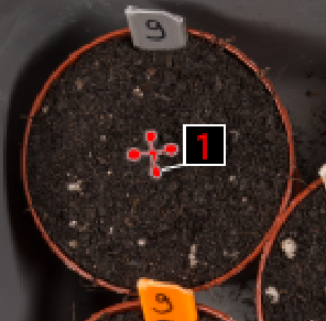
Thanks in advance for considering this!
Cheers Tijmen van Butselaar