Lesson 2: Data cleaning and production; SGD from scratch

[datalass1]

We start today's lesson learning how to build your own image classification model using your own data, including topics such as:

• Image collection
• Parallel downloading
• Creating a validation set, and
• Data cleaning, using the model to help us find data problems.

I'll demonstrate all these steps as I create a model that can take on the vital task of differentiating teddy bears from grizzly bears. Once we've got our data set in order, we'll then learn how to productionize our teddy-finder, and make it available online.

In the second half of the lesson we'll train a simple model from scratch, creating our own gradient descent loop. In the process, we'll be learning lots of new jargon, so be sure you've got a good place to take notes, since we'll be referring to this new terminology throughout the course (and there will be lots more introduced in every lesson from here on).

[datalass1]

Example Projects and plan for Lesson 2 (0-15mins)

Lots of interesting project examples, what will we learn and learn by doing motivation!

Help Jeremy create a classifier so that his daughter can identify teddy bears over grizzlys and black bears. (15mins-53mins)

Step1:

Search the images on Google Image

Step2:

Type Ctrl+Shift+J on the search page, the JavaScript console will appear, and paste: urls = Array.from(document.querySelectorAll('.rg_di .rg_meta')).map(el=>JSON.parse(el.textContent).ou); window.open('data:text/csv;charset=utf-8,' + escape(urls.join('\n')));

This script was inspired by Adrian Rosebrock Change name of the download file of urls to match the image class with .txt file type.

=# Step3:

Create directories for the imagery data on the GCP next to the lesson notebooks.

path = Path('data/bears')
dest = path/folder
dest.mkdir(parents=True, exist_ok=True)

Step4:

Scp the data (txt files) onto the GCP server

$ (base) ubuntu@ubuntu:~/git/fastai$ gcloud compute scp ~/Downloads/urls_grizzly.txt jupyter@my-fastai-instance:~/tutorials/fastai/course-v3/nbs/dl1/data/bears/grizzly/ 

$ (base) ubuntu@ubuntu:~/git/fastai$ gcloud compute scp ~/Downloads/urls_black.txt jupyter@my-fastai-instance:~/tutorials/fastai/course-v3/nbs/dl1/data/bears/black 

$ (base) ubuntu@ubuntu:~/git/fastai$ gcloud compute scp ~/Downloads/urls_teddys.txt jupyter@my-fastai-instance:~/tutorials/fastai/course-v3/nbs/dl1/data/bears/teddys

Step5: Run through notebook and train a model

Run through notebook lesson2-download. I have converted the download image from urls section and this is saved to GitHub as less2v3-download-20190202.pynb.

Get and look at data Start with GetDataBunch and have a look at some of the data.

Train model train the later layers, save model. unfreeze and find a good learning rate using:

leanr.lr_find()
learn.recorder.plot()

then fit the model for the earlier layers with the selected learning rates. save the model

look at the confusion matrix using ClassificationInterpretation object.

Step6: Clean out top losses/noisy data

Using top losses pick the images that the model is not confident of.

Using a widget delete or relabel data from validation and training datasets. Why writing applications in your notebooks are super useful for you fellow experimenters! :) It's not a great way to productionize, building a production webapp would be the best way to do this.

Step7: Production

You will want to run in production with a CPU. It's better for running a model, it might take longer, but it scales better.

Testing out single images on the model to make a prediction.

Starlette is very similar to flask.

Step8: Problems

Underfitting, overfitting: learning rate too low or too high, too few or too many epochs. What does this look like? High leanring rate: identified as the validation loss is much higher. Low learning rate: really slow loss changes as seen in plot_losses, learning rate too low. And for each epoch if the training loss is higher than the validation loss then it learning rate is too low. If the validation loss is still much lower than training loss then you havent trained your model enough, it's underfitting, Too few epochs: looks like too low a learning rate, underfitting. Too many epochs: When overfitting the model starts to recognise certain images in the dataset, so when seeing a new validation or test set the model won't be able to generalise well enough to get high accuracy. It is very difficult to overfit. It has taken many epochs, and overfitting can be recognised when the error_rate gets better then begins to get worse. If your training loss is lower than validation loss, this is NOT overfitting. It is a sign you have done something right. The model is overfitting when the error_rate is getting worse.

Let's look at what's going on! (53mins -

We will start seeing a little bit of math, using a number example (MNIST dataset). np.argmax will return a probability. ??learn.predict to see argmax being used in the source code.

Questions (55mins - 1hr01min):

1. Definition of how error rate is calculated. Try error_rate?? and what is accuracy?? and what is it being applied to whatever we pass through to metric parameter in create_cnn and this is applied to the validation dataset. doc(accuracy) to find out how to look at metrics documentation. Don't forget that the doc function is your friend.

2. Why were you using 3e-3 for learning rate? It seems to be a really good learning rate.

Back to the math (1hr01min - 1hr08min)

Adam Geitgey animated gif of the numbers.

This is a linear equation:

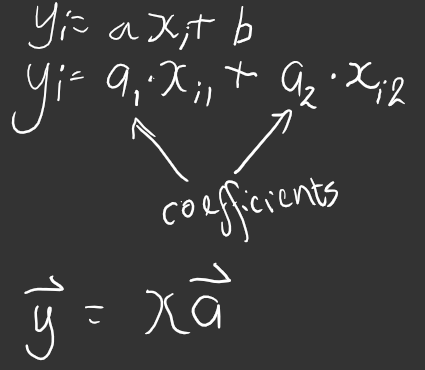
There are lots of values of y and lots of values of x. There are only ever one of the coefficients/parameters. One reason to do linear algebra, check out issue #23 but also to not write loops. So, when you have two things being multiplied together added to two things being multiplied together this is called a dot product so when you do this to a lot of numbers (i), then that's called a matrix product! The one vector y, is equal to one matrix called x, times one vector called a. Have a look at matrixmultiplication.xyz

Questions (1hr08mins - 1hr14mins)

1. When generating new image datasets, how do you know how many images are enough? You found a good learning rate. then you train for a long time and the error gets worse, and your still not happy with the accuracy. Get more data. Most of the time you need less data than you think. Get small amounts first.
2. What about unbalanced data? If you have 50 grizzlys and 100 teddys, it doesn't matter. No need to oversample.
3. Once you unfreeze and retrain and your training loss is still lower than your validation loss, do you retrain it unfrozen again, or do you re-do it all with a longer epoch? Do another cycle it may generalise a little better, if you start again, you could do either depend how patient you are.
4. About resnet34....basically resnet34 is an architecture it's a mathematical function.

Let's take a look at a basic neural network (1hr14mins -

We are looking at SGD which is a computer trying lots of things to come up with a really good function. Go to lesson2-sgd.pynb.

We have two coefficients 3 (slope) and 2 (intersect). They are wrapped up in a tensor. Tensor means array, an array of a regular/rectangle/cube shapes, e.g. 4 by 3 array is a tensor.
rank means dimensions.

Say to PyTorch that we want to create a tensor of n by 2. The number of rows will be n and the number of columns will be 2: x = torch.ones(n, 2) And for ever row of column 0 grab a uniform random number between -1 and 1 (in PyTorch the underscore means to replace rather than return): x[:,0].uniform_(-1,1) Create the parameters: a = tensor(3.,2) Now make the matrix product: y = x@a + torch.rand(n) Now make a scatted plot: plt.scatter(x[:,0], y);

So what does an equation with 50millions numbers look....like resnets coefficients. This is SGD!

Now let's pretend we don't know the values of the coefficients/parameters/weights. We want to minimise the error between the point and the line x@a. 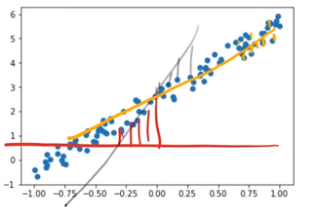The loss is the average of how far away the line is from all those points. As the loss decreases the line is a better fit. For regression the most common error function or loss function is the mean squared error. The value of the line (y) vs the actual prediction (y_hat).
so it is ((y_hat - y)2)/n aka ```((y_hat - y)2).mean()```

So what is the line. Let's guess. Then take the guess and make it better with gradient descent. There are two numbers, the intercept and the gradient of the line. The derivative will tell you whether moving it up or down make mse better or worse. Derivative aka gradient.

loss.backward calculates the derivative in the update function.

Then we look at learning rate. Demo with quadratic (1hr45mins)

Really cool animation in matplotlib to show SGD.

On a large dataset we use mini batches.

Vocab

Learning rate: the thing we multiple our gradient by to decide on how much to update the weight by Epoch: one complete run through all our data points. The more epochs we run the risk of overfitting. Minibatch: random bunch of points used to update weights SGD: gradient descent using minibatches Architecture/Model: The mathematical function you are fitting the parameters to Parameters/coefficients/weights: the number you are updating Loss: how far away you are from the correct answer.

Looking at overfitting (the higher degree polynomial) and underfitting. The way to make things fit just right is to use regularisation, so that when we train our model it works well on data it has seen and data that it hasn't seen (validation dataset). The validation set is really important, to hold back some data, check it on this data to see whether it generalises.