Lesson 5: Back propagation; Accelerated SGD; Neural net from scratch

[datalass1]

Overview

In lesson 5 we put all the pieces of training together to understand exactly what is going on when we talk about back propagation. We'll use this knowledge to create and train a simple neural network from scratch.

We'll also see how we can look inside the weights of an embedding layer, to find out what our model has learned about our categorical variables. This will let us get some insights into which movies we should probably avoid at all costs…

Although embeddings are most widely known in the context of word embeddings for NLP, they are at least as important for categorical variables in general, such as for tabular data or collaborative filtering. They can even be used with non-neural models with great success.

Great notes: https://forums.fast.ai/t/deep-learning-lesson-5-notes/31298

[datalass1]

Lesson 5: Back propagation; Accelerated SGD; Neural net from scratch

Foundations of Neural Nets! You need to use deep learning for computer vision for good results. Understanding more about regularisation to sort out underfitting.

This lesson uses EXCEL spreadsheets to support understanding of deep learning, with the example of collaborative learning.

There are only 2 types of layer: parameters and activations. 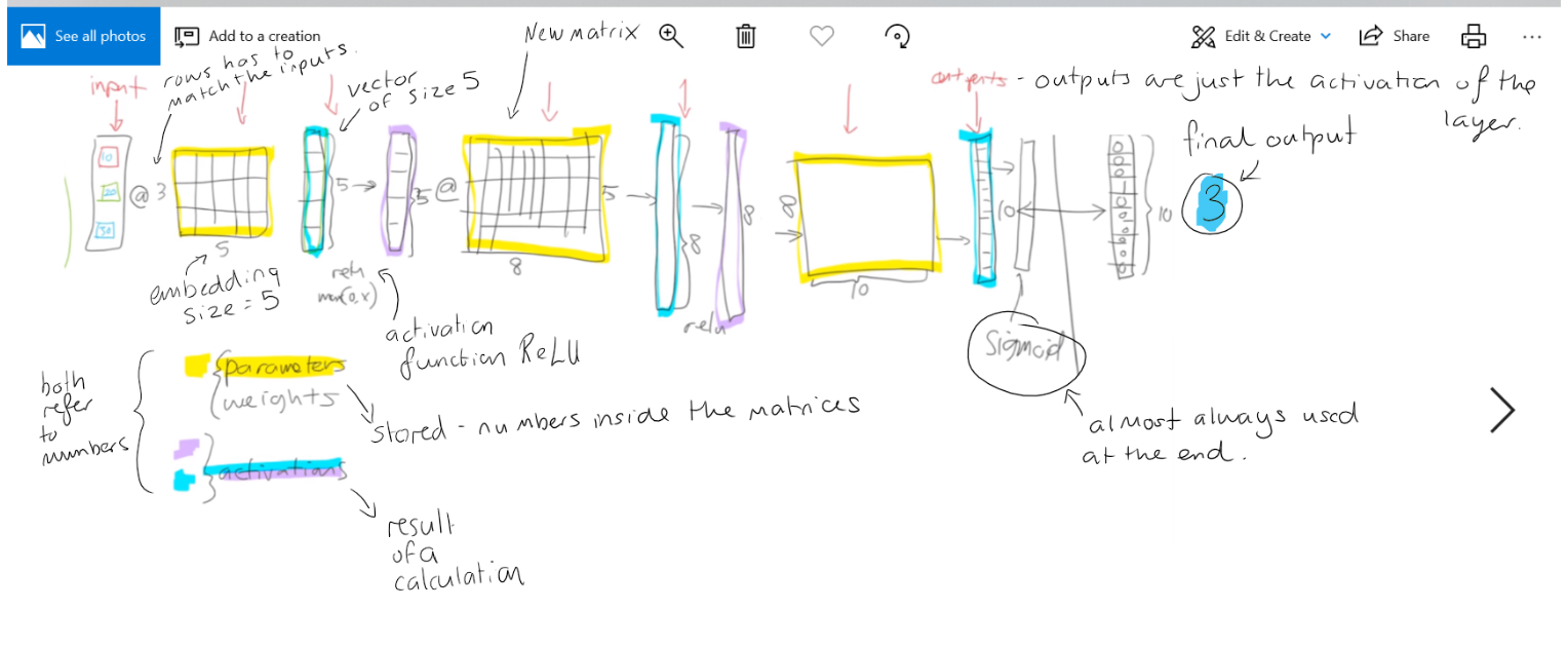The parameters are what you model learns. The yellow is our weight tensors/matrix, these numbers are calculated. Activations come from matrix multiplications (MM) and the activation funcions (in blue): an element wise function - a 20 long vector to 20 long activation. ReLU is what we normally use. MM followed by ReLU stacked together results is these amazing mathematical property called the universal approximation theorem which is if you have big enough weight matrices and enough of them it can solve any arbitrarily complex mathematical function to any arbitrarily high level of accuracy, assuming you can train the parameters time and compute.

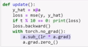
Back propagation

weights = weights - weights.grad * learning rate

Resnet34 has 1000 columns because there is 1000 images to classify in ImageNet. This weight matrix is no good in transfer learning. You have new categories to predict. So when you train a new cnn you delete the last layer and add new weight matrices (as big as you need it to be) with a new ReLU inbetween.

The Zeiler and Fergus paper is a good example of some of the things round in what a weight matrix will find. One of the filters can find corners, the next repeating patterns, next some round things etc, so the weight matrices are becoming more sophisticated, these weight are good so lets keep them as they are.

Don't bother training any of the other weights by freeze all the other layers. Then unfreeze and train the earlier layers, but not too much training. Discriminative learning rates.

Affine functions, it just means a linear function (like a MM, it is the most common kind of affine function used in deep learning). But as we’ll see when we do convolutions. Convolutions are matrix multiplications where some of the weights are tied and so it would be slightly more accurate to call them affine functions.

one hot encoding vs. array lookup aka embedding. Array lookup aka embedding is mathematically identical to doing a matrix product by a one-hot encoded matrix (24mins). Always do an array lookup/embedding - it is much faster and memory efficient.

latent features once we train a neural net

bias we can add another row to the matrix for MM which will take into account bias. Better model and better result, makes sense semantically.

Helpful HINT if you get this error, this means that csv isn’t unicode. We solve this by adding encoding='latin-1'

movies = pd.read_csv(path/'u.item',delimite='|', encoding='latin-1', 
         header=None, names=['movieId','title','date','N','url',*
         [f'g{i}' for i in range(19)]])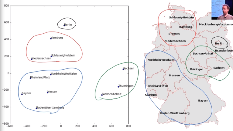

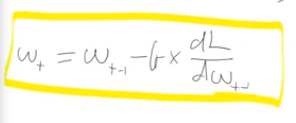[datalass1]

Entity Embeddings of Categorical Variables (1hr07mins)

Cheng Gus and Felix Berkhahn Discovering geography:

Weight Decay (1hr13mins)

With too many parameters the model is overfitting and not generalising well. Why can't I have lot's of parameters? You can. It's a fiction that too many parameters is bad. More parameters mean more non-linearity, like life.

One way to penalize the complexity is, to sum up the square of the parameters. Then we just add that number to the loss. But there is the problem that sum can be so big that it is better for the model to just set all parameters into zero. That is why we multiply the sum with some small hyperparameter. In Fastai that is called wd (weight decay) which generally should be 1e-1. People test a different kind of numbers instead of 1e-1 but it seems to be working best. By default in Fastai library, the weight decay is 1e-2 It is less than it should because in rare cases too big weight decay is causing that model doesn’t learn and that might cause hard to recognize problem for beginners. Jeremy recommends using 1e-1 instead of the default because now when you understand that if parameters become zero then the weight decay is too high.

Stochastic Gradient Descent

Look at lesson-sgd nb and refresh with lesson 2.

HINT x_train,y_train,x_valid,y_valid = map(torch.tensor,(x_train,y_train,x_valid,y_valid)) instead of

x_train = torch.tensor(x_train)
y_train = torch.tensor(y_train)
x_valid = torch.tensor(x_valid)
y_valid = torch.tensor(y_valid)

Be comfortable with this equation/code(highlighted part). Basically, new weights/parameters are calculated by taking the previous epochs weights (time -1) subtract the learning rate, times the derivative of the loss function divided by the derivative of weight (time -1).

Weight decay: good to be conservative with weight decay, set as 0.01

So whats our loss, the dL? It's a function of our independent variables (x) and our weights = mse(predictions, actuals). Predictions are model(predictions, weights). We are also going to add weight decay, which is 0.1 times the sum of weights squared.

Demo this using MNIST: as a standard fully connected net.

See nb for all tutorial notes PyTorch is going to do a lot of the work for us.

Learn how to subclass! (1hr29mins)

class Mnist_Logistic(nn.Module):
    def __init__(self):
        super().__init__()
        self.lin = nn.Linear(784, 10, bias=True)

    def forward(self, xb): return self.lin(xb)

We want to create an attribute in our class which contains a linear layer: the nn.Linear. It does: y_hat = x@a Why don't you create a PyTorch linear background?

Logistic regression model first, it is a one layer neural net.

Back in excel to demo gradient descent: Start off with randomly generated x and y data for ax+b. a=2 b=30 Every row is a batch size of 1. y_pred: Starting with intercept and slope of 1, the first prediction for x=14 and y=58 is 15. Calculated by 1*14+1 (ax+b).

Calculate Loss (with finite differencing) : err^2: is y-y_pred^2. So (58-15)^2 = 1,849.00 aka the square error. errb1: what is the gradient? (((intercept + 0.01) + xslope) - y)^2. So ```(((1+0.01) + 141)-58)^2 = 1,848.14 *est de/db*: so our derivative is the difference in loss divided by 0.01. (errb1-err^2)/0.01. So(1,848.14 - 1,849.00)/0.01 = 85.99```

erra1: (((intercept + 0.01) x + slope) - y) ^ 2. So ```(((1+0.01) 14 = 1)-58) ^ 2 = 1,836.1225 *est de/da*: (erra1-err^2)/0.01. So(1,836.1225 - 1,849)/0.01 = 1,202.04 *de/db*: 2*(y_pred - y). So2 (15 - 58) = -86.00``` de/da: de/db x. So -86 * 14 = -1,204

So gradient descent: new a: slope - de/da learning rate. So ```1 - (-1,204 0.0001) = 1.12 *new b*: intercept - de/db * learning rate. So1 - (-86 * 0.0001) = 1.01```

Keep on doing this until completing one epoch. This is REALLY slow.

Dynamic Learning Rates

Let's add momentum.

Adding momentum the current gradient plus the exponentially weighted moving average of the past few steps. It's normally 0.9.

Homework: Take lesson 2 SGD and add momentum.

RMSprop: Think of Geoffrey Hinton on the coursera online MOOC is where it first appeared. It is very similar to momentum, with the gradient squared.

Adam: Keeping track of the exponentially weighted average of gradient AND steps: momentum and rmsprop.

Finally, understanding Tabular Data

Adult dataset about who makes more money.

what cross entropy loss is

ml cheatsheet You will normally want softmax as the actiavtion function and cross entropy as the loss