 datalass1
commented
5 years ago
datalass1
commented
5 years ago Building a Deep Learning Architecture from scratch with MNIST using resnet
Our image item list contains 70,000 items, and it's a bunch of images that are 1 by 28 by 28.
Once you've got an image item list, you then split it into training versus validation.
Next thing we can do is to add transforms; for small images of digits like this, you just add a bit of random padding.
Now we've got a transformed labeled list, we can pick a batch size and choose data bunch.
We can choose normalize. In this case, we're not using a pre-trained model, so there's no reason to use ImageNet stats here. So if you call normalize like this without passing in stats.
Basic CNN with batch norm
Normalization is a process where given a set of data, you subtract from each element the mean value for that data set and divide it by the data set's standard deviation. By doing so, we put the input values onto the same "scale".
Often times with images, we don't worry about dividing by the standard deviation, but just subtract the mean.
Let's start out creating a simple CNN. The input is 28 by 28.
All of my convolution is going to be kernel size 3 stride 2 padding 1.
def conv(ni,nf): return nn.Conv2d(ni, nf, kernel_size=3, stride=2, padding=1)
Each time you have a convolution, it's skipping over one pixel so it's jumping two steps each time. That means that each time we have a convolution, it's going to halve the grid size.
model = nn.Sequential(
    conv(1, 8), # 14
    nn.BatchNorm2d(8),
    nn.ReLU(),
    conv(8, 16), # 7
    nn.BatchNorm2d(16),
    nn.ReLU(),
    conv(16, 32), # 4
    nn.BatchNorm2d(32),
    nn.ReLU(),
    conv(32, 16), # 2
    nn.BatchNorm2d(16),
    nn.ReLU(),
    conv(16, 10), # 1
    nn.BatchNorm2d(10),
    Flatten()     # remove (1,1) grid
)
We've got a grid size of one now. It's not a vector of length 10, it's a rank 3 tensor of 10 by 1 by 1. Our loss functions expect (generally) a vector not a rank 3 tensor, so you can chuck flatten at the end, and flatten just means remove any unit axes.
That's how we can create a CNN. Then we can return that into a learner by passing in the data and the model and the loss function and optionally some metrics. We're going to use cross-entropy as usual. We can then call learn.summary() and confirm.
learn = Learner(data, model, loss_func = nn.CrossEntropyLoss(), metrics=accuracy)
learn.summary()
We can grab that mini batch of X that we created earlier (there's a mini batch of X), pop it onto the GPU, and call the model directly.
xb = xb.cuda()
learn.lr_find(end_lr=100)
learn.recorder.plot()
learn.fit_one_cycle(3, max_lr=0.1)
We get 98.6% accuracy.
Refactor
fast.ai already has something called conv_layer which lets you create conv, batch norm, ReLU combinations.
def conv2(ni,nf): return conv_layer(ni,nf,stride=2)
model = nn.Sequential(
    conv2(1, 8),   # 14
    conv2(8, 16),  # 7
    conv2(16, 32), # 4
    conv2(32, 16), # 2
    conv2(16, 10), # 1
    Flatten()      # remove (1,1) grid
)
I've created the same neural net, with less code.
learn = Learner(data, model, loss_func = nn.CrossEntropyLoss(), metrics=accuracy)
learn.fit_one_cycle(10, max_lr=0.1)
More cycles, and the model is 99.1% accurate.
ResNet-ish
Influential paper: Deep Residual Learning for Image Recognition by Kaiming He and colleagues at (then) Microsoft Research.
They looked at training error:
 The deeper layer did not overfit. It was worse than the shallower network.
So he made a new version of the 56 layer network by doing this:
The deeper layer did not overfit. It was worse than the shallower network.
So he made a new version of the 56 layer network by doing this:
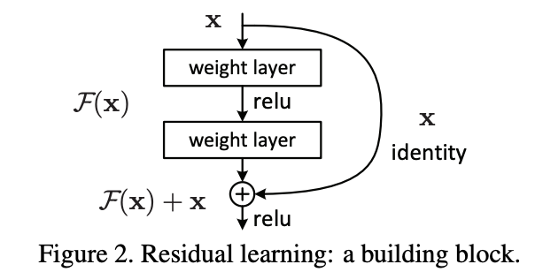 Every two convolutions adding together the input to those two convolutions.
Output = x + Conv2(Conv1(x))
So this thing here is (as you see) called an identity connection. It's also known as a skip connection.
A 56 layer neural network without skip connections is very very bumpy.
 This is discussed in Visualizing the Loss Landscape of Neural Nets
Now include the res_block:
class ResBlock(nn.Module):
    def __init__(self, nf):
        super().__init__()
        self.conv1 = conv_layer(nf,nf)
        self.conv2 = conv_layer(nf,nf)

    def forward(self, x): return x + self.conv2(self.conv1(x))
although a res block function already exists in fastai res_block, so use that.
model = nn.Sequential(
    conv2(1, 8),
    res_block(8),
    conv2(8, 16),
    res_block(16),
    conv2(16, 32),
    res_block(32),
    conv2(32, 16),
    res_block(16),
    conv2(16, 10),
    Flatten()
)
Keep refactoring
def conv_and_res(ni,nf): return nn.Sequential(conv2(ni, nf), res_block(nf))
model = nn.Sequential(
    conv_and_res(1, 8),
    conv_and_res(8, 16),
    conv_and_res(16, 32),
    conv_and_res(32, 16),
    conv2(16, 10),
    Flatten()

)
Results in an accuracy of 99.54%
U-net
They are particularly useful in other places in other ways of designing architectures for segmentation.
 The left half is called the downsampling path look like. Ours is just a ResNet 34.
So how do we double the grid size? We do a stride half conv, also known as a deconvolution, also known as a transpose convolution.
There is a fantastic paper called A guide to convolution arithmetic for deep learning that shows a great picture of exactly what does a 3x3 kernel stride half conv look like.
This is how you can increase the resolution.
And it's kind of obvious it's a dumb way to do it for a couple of reasons. When you get down to that 3x3 area, 2 out of the 9 pixels are non-white, but this left one, 1 out of the 9 are non-white. So there's different amounts of information going into different parts of your convolution. So it just doesn't make any sense to throw away information like this and to do all this unnecessary computation and have different parts of the convolution having access to different amounts of information.

Why not just do this?
 TO set up there is no compution. But then you could do a stride 1 conv, and now you've got values and computation.
Another approach is instead of using nearest neighbour interpolation, you can use bilinear interpolation which basically means instead of copying A to all those different cells you take a weighted average of the cells around it.
A useful blog: https://towardsdatascience.com/understanding-semantic-segmentation-with-unet-6be4f42d4b47
Overview In the final lesson of Practical Deep Learning for Coders we'll study one of the most important techniques in modern architectures: the skip connection. This is most famously used in the resnet, which is the architecture we've used throughout this course for image classification, and appears in many cutting edge results. We'll also look at the U-net architecture, which uses a different type of skip connection to greatly improve segmentation results (and also for similar tasks where the output structure is similar to the input).
We'll then use the U-net architecture to train a super-resolution model. This is a model which can increase the resolution of a low-quality image. Our model won't only increase resolution—it will also remove jpeg artifacts, and remove unwanted text watermarks.
In order to make our model produce high quality results, we will need to create a custom loss function which incorporates feature loss (also known as perceptual loss), along with gram loss. These techniques can be used for many other types of image generation task, such as image colorization.
Finally, we'll learn about a recent loss function known as generative adversarial loss (used in generative adversarial networks, or GANs), which can improve the quality of generative models in some contexts, at the cost of speed.
The techniques we show in this lesson include some unpublished research that:
Let us train GANs more quickly and reliably than standard approaches, by leveraging transfer learning Combines architectural innovations and loss function approaches that haven't been used in this way before. The results are stunning, and train in just a couple of hours (compared to previous approaches that take a couple of days).