binseg not expected/optimal speed for best case data

[tdhock]

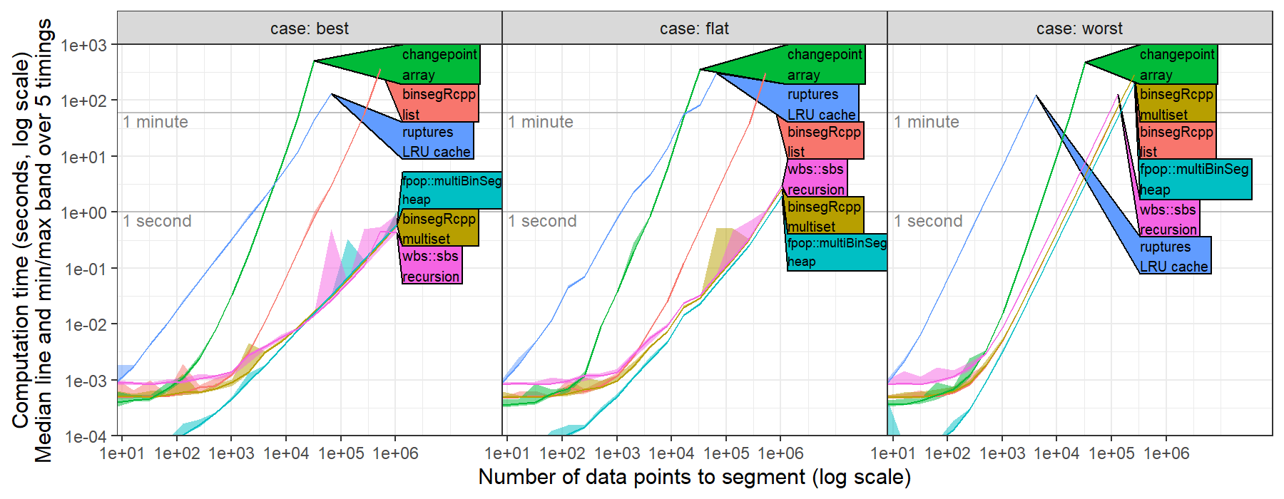
related to benchmarks #231 I recently computed timings for ruptures.Binseg using the l2 model (normal change in mean, square loss) for univariate data, https://github.com/tdhock/binseg-model-selection#22-mar-2022 For worst case data, ruptures shows the expected/optimal quadratic time complexity. For best case data, ruptures was slower than the expected/optimal log-linear time complexity. This is probably because the time complexity of CostL2.error(start,end) is linear in number of data, O(end-start). Could probably be fixed by computing cumsum vectors in fit method, then using them to implement a constant O(1) time error method.

[deepcharles]

Hi, indeed using Dynp(model="l2") results in a O(log(T^3)) complexity where T is the number of samples. Using precomputed cumsum vectors will definitely make it faster.

The fastest way to detect mean-shifts is to use KernelCPD(kernel="linear"). It follows this article and is coded in C. The complexity is quadratic in number of operations and linear in memory.

See here for a comparison between the Python implementation and the C implementation.

[deepcharles]

Hi,

You can try the following cost function which implements CostL2 with pre-computed cumsum signals. Hopefully, it will show the expected/optimal log-linear time complexity.

The following code defines the cost function.

from ruptures.costs import NotEnoughPoints

from ruptures.base import BaseCost
import numpy as np
from numpy.linalg import norm

class CostL2CumSum(BaseCost):

    r"""
    Least squared deviation.

    For two indexes $a<b$, the cost function on the sub-signal
    $y_{a..b} = [y_a, y_{a+1},\dots,y_{b-1}]$, is equal to

    $$
     c(y_{a..b}) = \sum_{t=a}^{b-1} \|y_t - \bar{y}_{a..b}\|^2
    $$

    where $\bar{y}_{a..b}$ is the empirical mean of $y_{a..b}$.

    For efficiency, the cost function is re-written with the cumulative sums of
    the signals $y$ and $[\|y_1\|^2, \|y_2\|^2,\dots,\|y_T\|^2]$.
    """

    model = "l2_cumsum"

    def __init__(self):
        """Initialize the object."""
        self.signal = None
        self.signal_cumsum = None
        self.signal_norm_cumsum = None
        self.min_size = 1

    def fit(self, signal) -> "CostL2":
        """Set parameters of the instance.

        Args:
            signal (array): array of shape (n_samples,) or (n_samples, n_features)

        Returns:
            self
        """
        if signal.ndim == 1:
            self.signal = signal.reshape(-1, 1)
        else:
            self.signal = signal

        self.signal_cumsum = np.cumsum(self.signal, axis=0)
        self.signal_norm_cumsum = np.cumsum(norm(self.signal, axis=1) ** 2, axis=0)

        return self

    def error(self, start, end) -> float:
        """Return the approximation cost on the segment [start:end].

        Args:
            start (int): start of the segment
            end (int): end of the segment

        Returns:
            segment cost (float): the value of the cost on the segment [start:end]

        Raises:
            NotEnoughPoints: when the segment is too short (less than `min_size`
            samples).
        """
        if end - start < self.min_size:
            raise NotEnoughPoints

        if start == 0:
            res = self.signal_norm_cumsum[end - 1] - norm(
                self.signal_cumsum[end - 1]
            ) ** 2 / (end - start)
            return res
        res = (
            self.signal_norm_cumsum[end - 1]
            - self.signal_norm_cumsum[start - 1]
            - norm(self.signal_cumsum[end - 1] - self.signal_cumsum[start - 1]) ** 2
            / (end - start)
        )
        return res

To use it with Binseg

algo = rpt.Binseg(custom_cost=CostL2CumSum(), jump=1, min_size=1).fit(signal)
algo.predict(n_bkps=10)

[deepcharles]

We will not change the current implementation of CostL2 because, for small signals (below 1000 samples approx.), the naive implementation is faster.

Hope this helps

[deepcharles]

Closing for now, feel free to reopen.

[tdhock]

thanks for sharing your CostL2CumSum class. I re-ran my timings using that method. I observed about the same asymptotic timings using the new method (displayed as ruptures cumsum in figure) as the old method (displayed as ruptures l2). This result suggests that some other property of ruptures (not the l2 cost function) is the source of the slowdown. (maybe the storage of previously computed splits in the LRU cache?)

[tdhock]

Additionally I observed that the new CostL2CumSum class does not compute the same segmentation as the l2 cost. Figure below shows that the two methods result in segmentations with different loss/cost values. This is using

Python 3.7.6 | packaged by conda-forge | (default, Jun  1 2020, 18:11:50) [MSC v.1916 64 bit (AMD64)] on win32
Type "help", "copyright", "credits" or "license" for more information.
>>> import ruptures
>>> ruptures.version.version
'1.1.6'

[deepcharles]

new CostL2CumSum class does not compute the same segmentation as the l2 cost.

Hum, I fear that for such long signals, the cumsum vectors quickly overflow but that is only an assumption. To cope with this, they should be replaced by cumulative average.

If that still interests you, I can provide the associated cost function.

[deepcharles]

I observed about the same asymptotic timings using the new method (displayed as ruptures cumsum in figure) as the old method (displayed as ruptures l2).

I do not know why to be honest. Is the number of changes fixed?

[tdhock]

No the number of changes is not fixed. In the experiment https://github.com/tdhock/binseg-model-selection/blob/main/figure-timings-data.R I used

  max.segs <- as.integer(N.data/2)
  max.changes <- max.segs-1L

so it should be log-linear in N.data in the best case.