 kalebentley
commented
4 years ago
kalebentley
commented
4 years ago Hi Eric,
Thanks for the email. I’ve provided a few quick responses below. Also, I forwarded your email to Thomas and he provided a brief response that I’ve pasted in below, as well.
- NAs – I think your “judgment calls” regarding NAs are right. Looking at the raw data, your logic makes sense.
- Missing earlier estimates - I noticed this morning that there are (likely) missing estimates of abundance. First, there should be some estimates for 2001 and there are currently none. Second, as you pointed out, there are some instances where NAs are listed for total abundance but biodata exists. I quickly chatted with Todd Hillson this morning and, in short, he said there are some “issues” with estimates from earlier years. We may be able to track down some of these estimates and update the Spawner Abundance .csv file. Curious – as we work on updating the file, would it be helpful (or ok) if we tried to “fix” the zero vs. NAs?
- Populations – you updated “Population2” seems fine to me and matches the scale at which the estimates are generated.
- Densities – I need to get you population-specific estimates of spawning habitat. Curious, is there a specific unit (length, area) you would want these in? Also, does the model allow these units to change by year? I can work on getting these estimates to you ASAP – do you have a specific date when you would want them?
If it would be helpful, we could plan on having a check-in phone call sometime soon to discuss any remaining issues, results, and next steps.
Kale
*** Here’s Thomas’ email:
A couple quick comments without fully diving in:
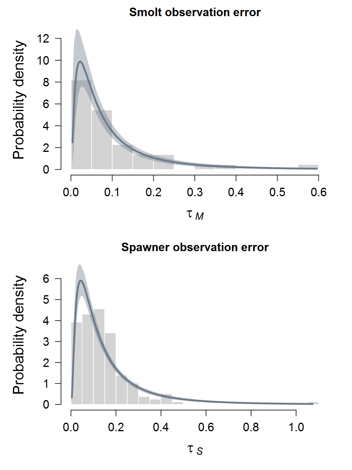
- Surprised estimated spawners diverge so much from observed spawners…with our observation error estimates being generally very low (CV ~ 5% often), would have thought they would have matched closer…do these results actually make use of the observation error estimates? If so, as priors or fixed?
- Productivity parameter modeled hierarchically makes sense either for 1 stage model… for 2 stage model could explore a mixed model:
log(alpha_freshwater) = mu + XB + eps
where: mu is the grand mean XB is a design matrix of habitat “types” (mainstem, constructed spawning channel, off channel). Betas could be modeled as random effect. eps ~ N(0, sigma) is a population specific residual from the mixed model
and
log(alpha_ocean) = mu + XB + eps mu is the grand mean X is a column with the distance from the ocean by population and B is a coefficient describing the effect of distance from river mouth on average marine survival eps ~ N(0, sigma) is a population specific residual from the mixed model
- capacity parameter I believe can be modeled as a mixed model:
log(capacity) = mu + log(km^2 of habitat) + eps
where: mu is the grand mean log(km^2 of habitat) is an offset term (you need to supply a coarse estimate of available (as opposed to used) spawning habitat…I can review these with you eps ~ N(0, sigma) is a population specific residual from the mixed model
The rationale for the models above is that productivity in the two stage model can be divided into freshwater and ocean…the freshwater part could be explained by habitat type, which affects max egg to fry survival (productivity) and spawning habitat quantity (capacity), where as the saltwater component could be affected by distance from the ocean (if fry take a beating in the Columbia, the further up they are).
Misc questions:
- how are you dealing with harvest removals? (todd may have estimates over time…yes minimal but may wish to include, particularly if they differentially affect pops)
- how are you dealing with broodstock removals or importation of spawners/eggs/fry from other pops (Duncan Channels, Grays hatchery)?
- Recruitment process errors…are these being modeled as an AR1 model? Univariate or multivariate? If multivariate, spatial or non-spatial prior? Would recommend multivariate…maybe start with non-spatial prior (LKJ for correlation matrix?)…when 2 stage model, maybe good to discuss modeling process error residuals among populations....gets trickier/more options… Are we eventually going to include hatchery pops? How ?
 ebuhle


 Hillsont

Hi @kalebentley, sorry this has taken so long. The data wrangling turned out to be nontrivial; I kept encountering unanticipated wrinkles and did a lot of iterating between data cleaning and model fitting with strange results that eventually pointed back to data issues, etc. I'm working on a RMarkdown vignette, but I wanted to put some preliminary results up here for discussion ASAP.
First, let me run through the key decisions / assumptions I made in data cleaning and ask you if they make sense. The following points relate to the spawner abundance data.
In a number of cases, I had to decide whether observations (
Abund.Mean) coded asNAwere truly missing or were actually zeros. A typical scenario would be a naturally spawning population with broodstock removals (i.e., "hatchery" dispositions), where natural spawner abundance and/or one or more broodstock dispositions wereNAin some years. In such cases, summing the natural spawners and broodstock removals to getS_obs(total returning adults) would obviously returnNA. This resulted in an awful lot of missing values. The problem was most acute for Duncan Creek, where I think there were only 2 years with non-missingS_obs. To deal with this, I made some judgment calls:NAs in hatchery dispositions (including Duncan Channel) are really zeros. I reasoned that the number of fish taken for broodstock should always be recorded, and in most cases it was.NAs in Duncan Creek from 2004-present are really zeros. Since there is a weir, I assumed we knew the number of returning adults and where they ended up (Duncan Creek, Duncan Channel, or Duncan Hatchery) every year once monitoring started. There were no non-missing values for any disposition until 2004, so I assumed that was the start of the time series.NAs in natural spawner abundance are real missing observations.I excluded all cases with leading
NAs inS_obseven when (to my surprise) there were BioData available. Missing spawner abundance in the initial1:max_ageyears of a time series causes problems for model fitting because there are obviously no earlier data to constrain the process model of recruitment. Initial states are given diffuse priors, and typically the process-model information flowing backward from later data is insufficient to identify them. I gave it a shot anyway, since some populations have age- and origin-composition data starting before the spawner abundance series (but of course the compositional data don't inform the absolute scale, just relative cohort strength). The resulting fits were a disaster, to use the technical term, so I trimmed the leadingNAs and things became much better-behaved.Finally, I ended up departing from the mapping of
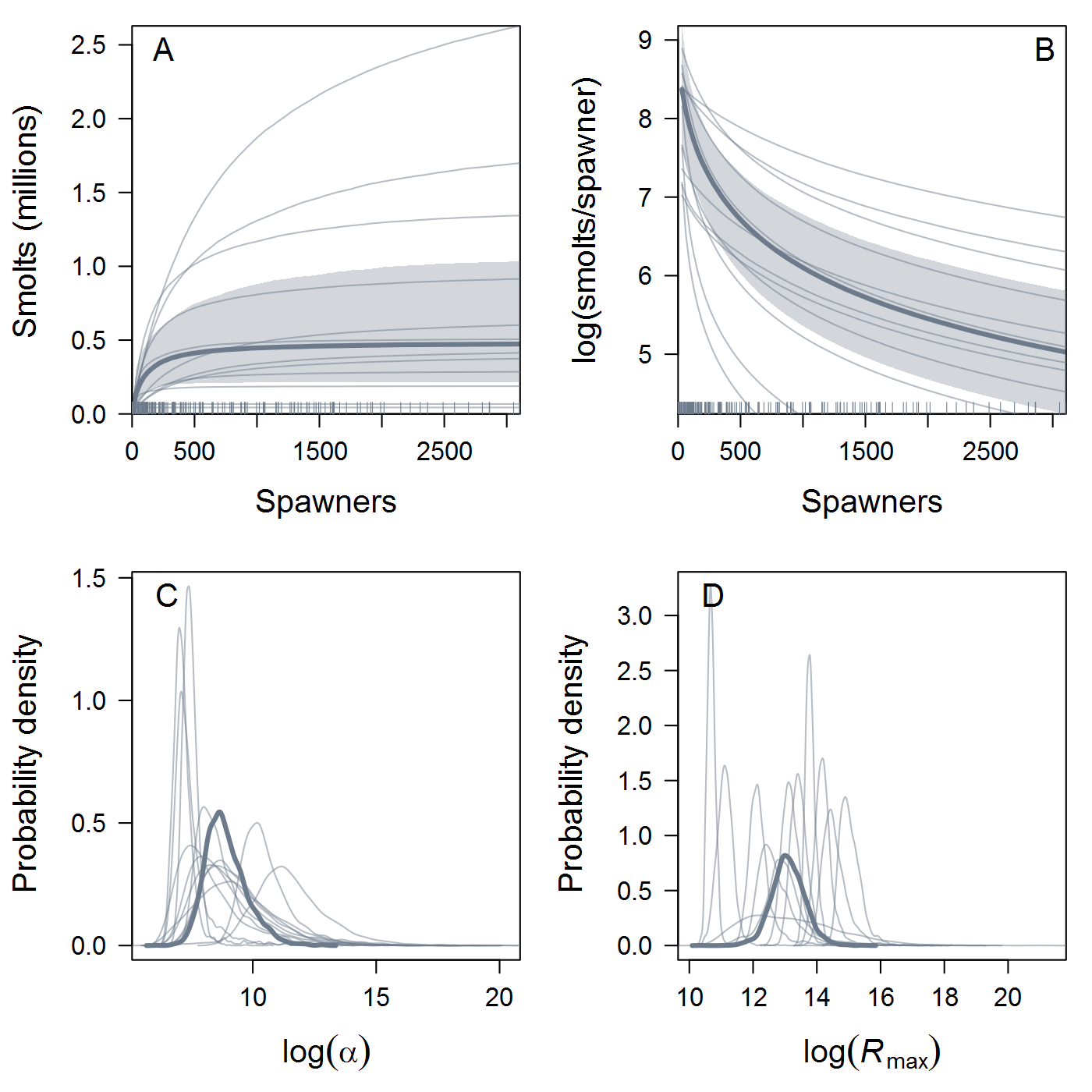
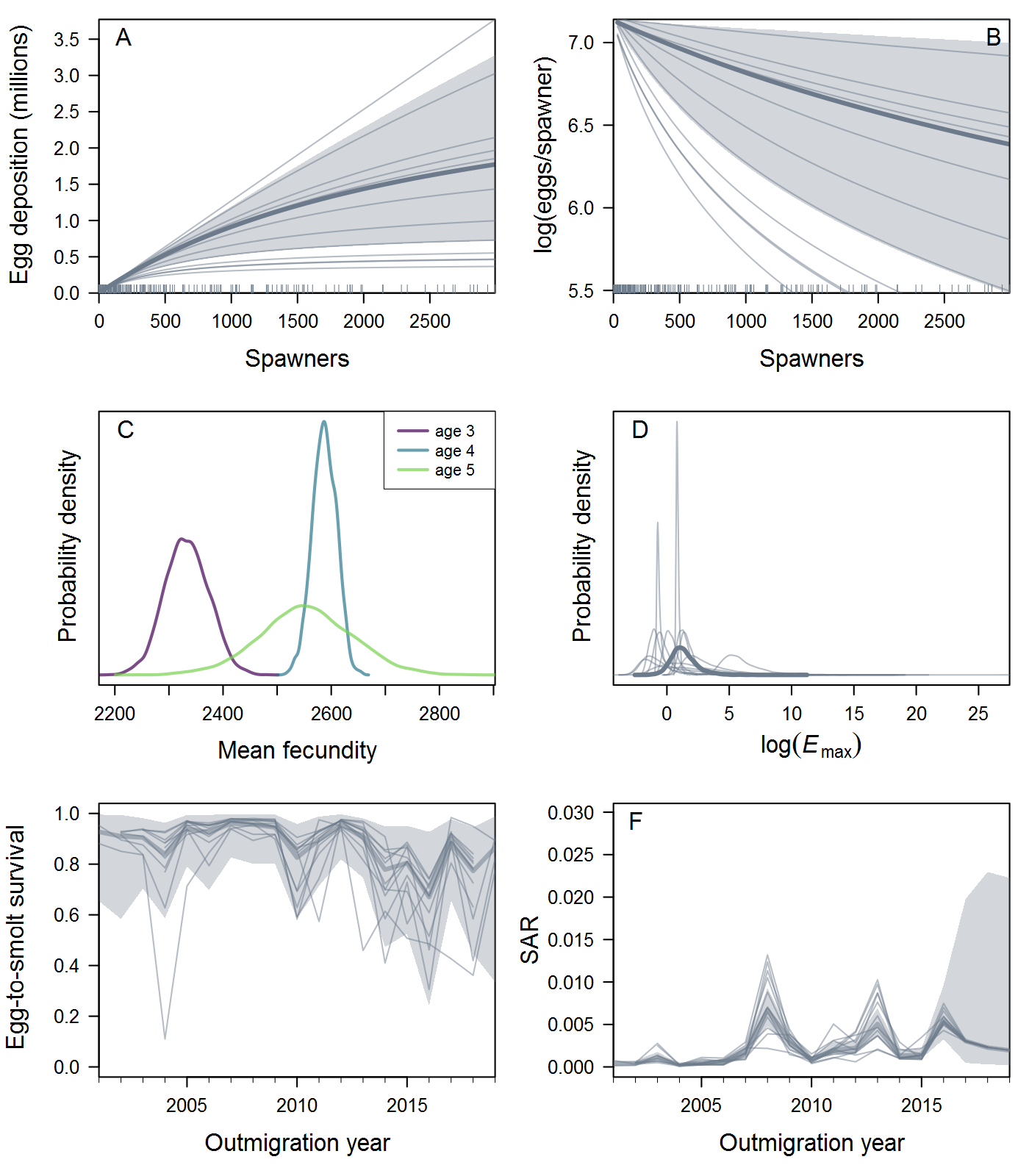
Location.Reachtopopthat you proposed. I first tried your 8 populations (Population1in the table below) but ran into computational problems (terrible mixing, lots of divergences, etc.) that weren't resolved by the usual Stan techniques. Eight is a pretty small number of groups for hierarchical modeling, so I tried a more "splitty" grouping with 12 populations (Population2) and got much more stable and sensible results. This could be a case of Gelman's folk theorem, or it could just be luck (Stein's paradox and all that). Either way, the results shown below are based on the 12-population data.All that said, here are some results, finally! I fit spawner-to-spawner IPMs with three candidate spawner-recruit functions: exponential, Beverton-Holt, and Ricker. I haven't done formal model comparison using LOO yet, but we can see immediately that the B-H fit is somewhat dubious -- it's basically flat over the range of the data, with very (implausibly?) high intrinsic productivity. In the left panel, the thick curve and shaded 95% credible interval are the ESU-level or hyper-mean S-R relationship, and the thin curves are posterior medians for each of the 12 populations. Similarly, the posterior distribution of intrinsic productivity (
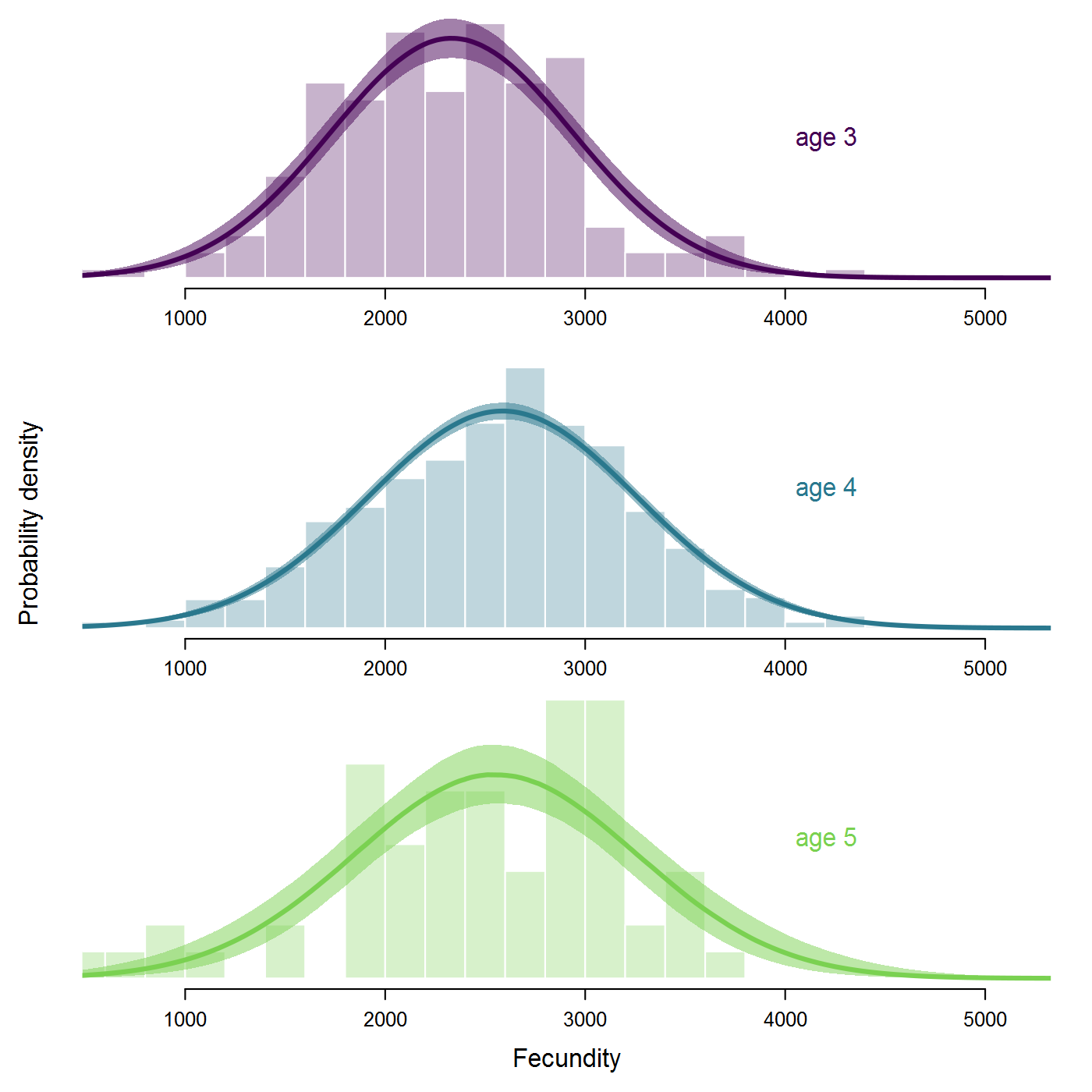
alpha) and maximum recruitment (Rmax, in units of spawners) are shown for the ESU and individual populations.The Ricker estimates look more reasonable, although the S-R curve doesn't approach overcompensation in the estimated range of spawner abundance. As expected, the Ricker produces much lower estimates of intrinsic productivity than the B-H, including a 17% probability that the growth rate is actually negative at the ESU level. Some populations have bimodal posterior distributions of
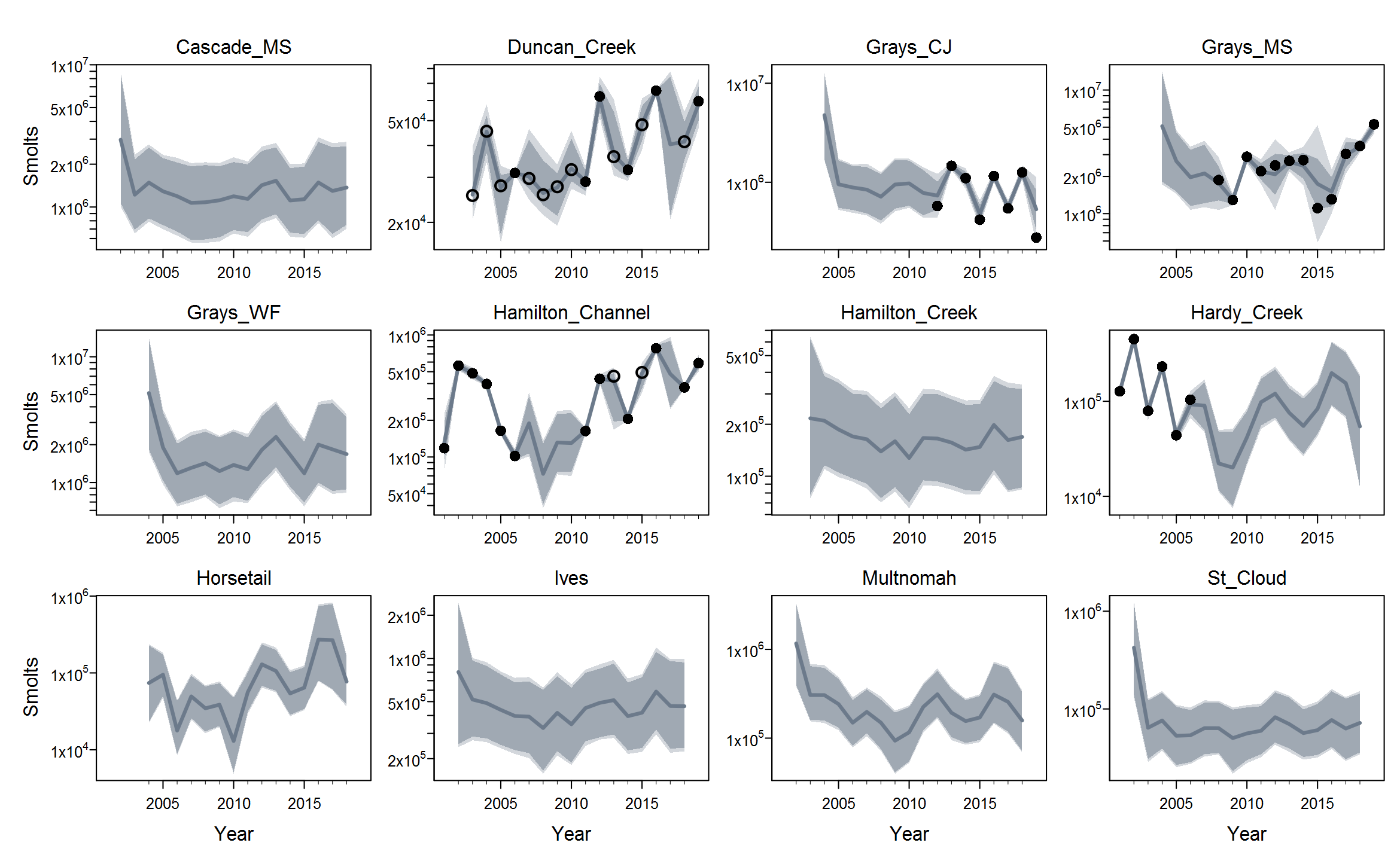
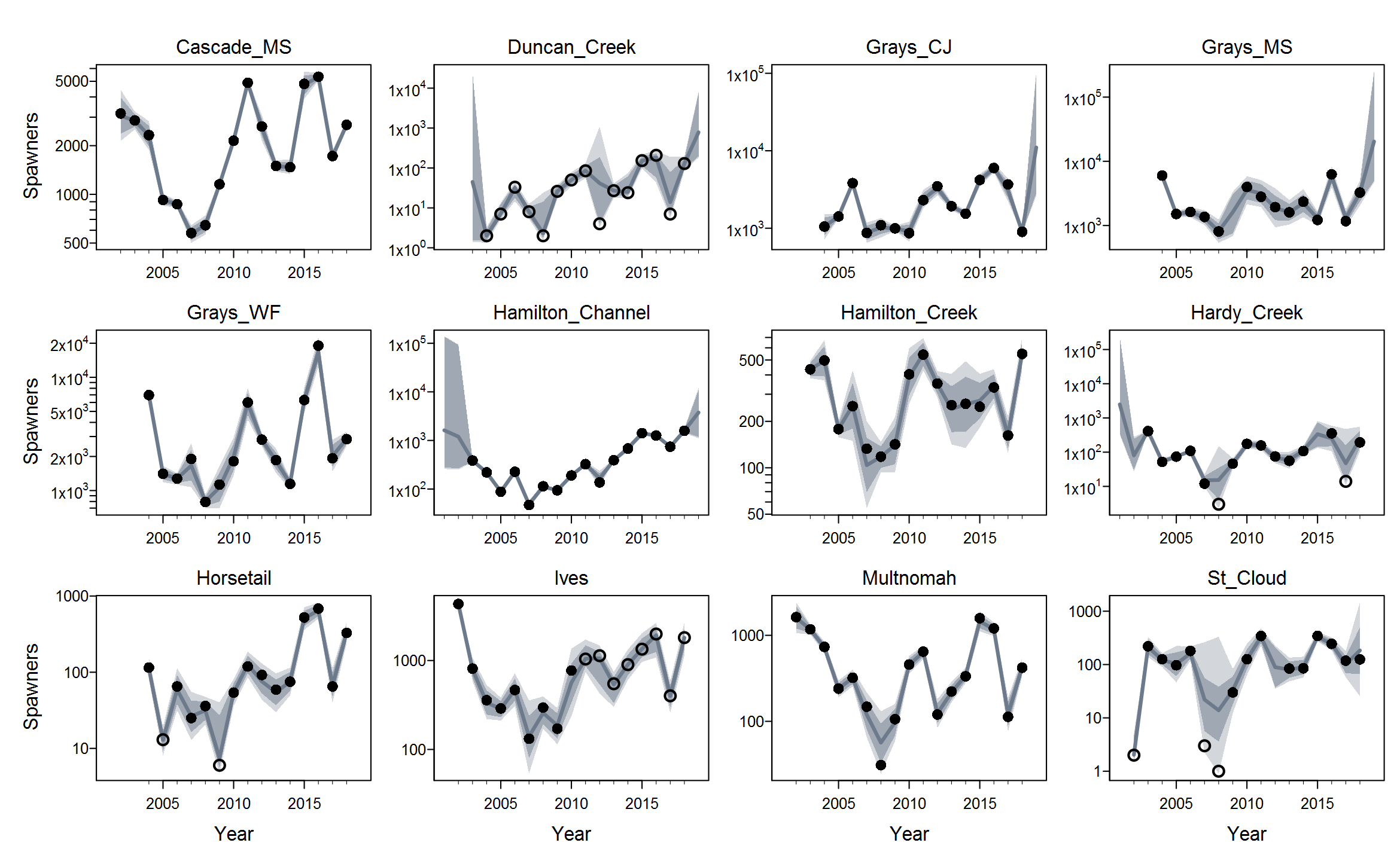
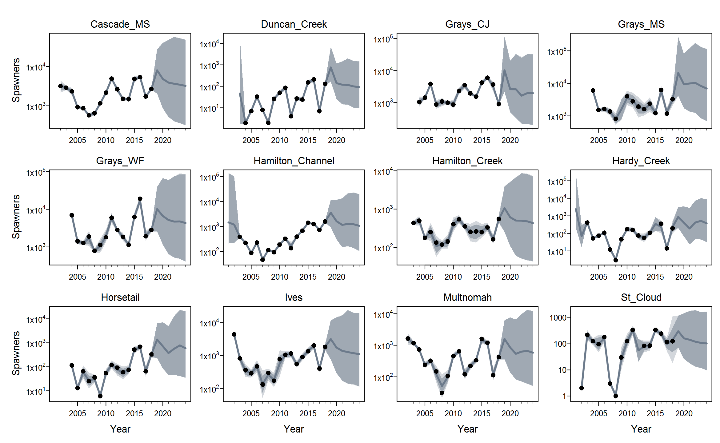
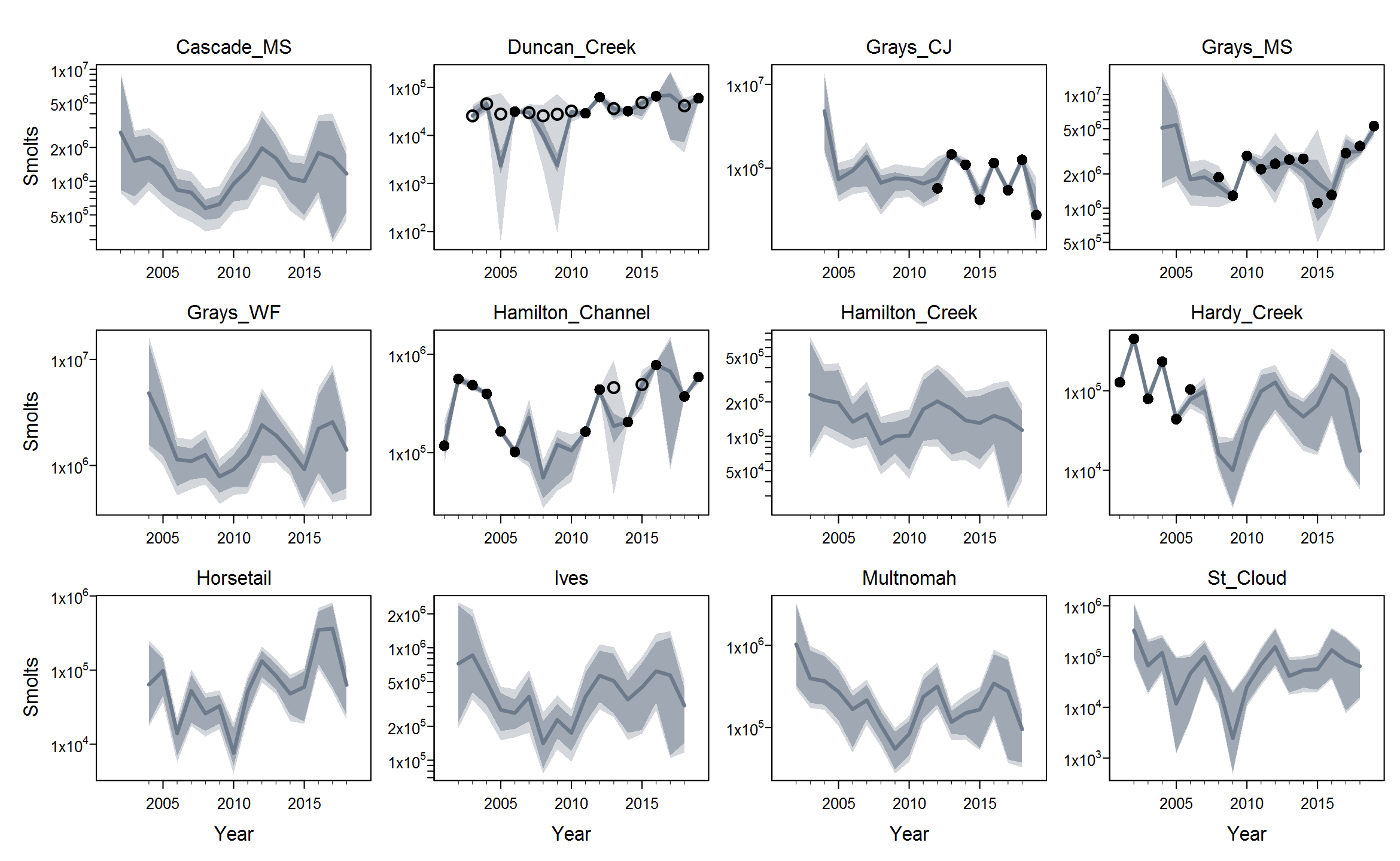
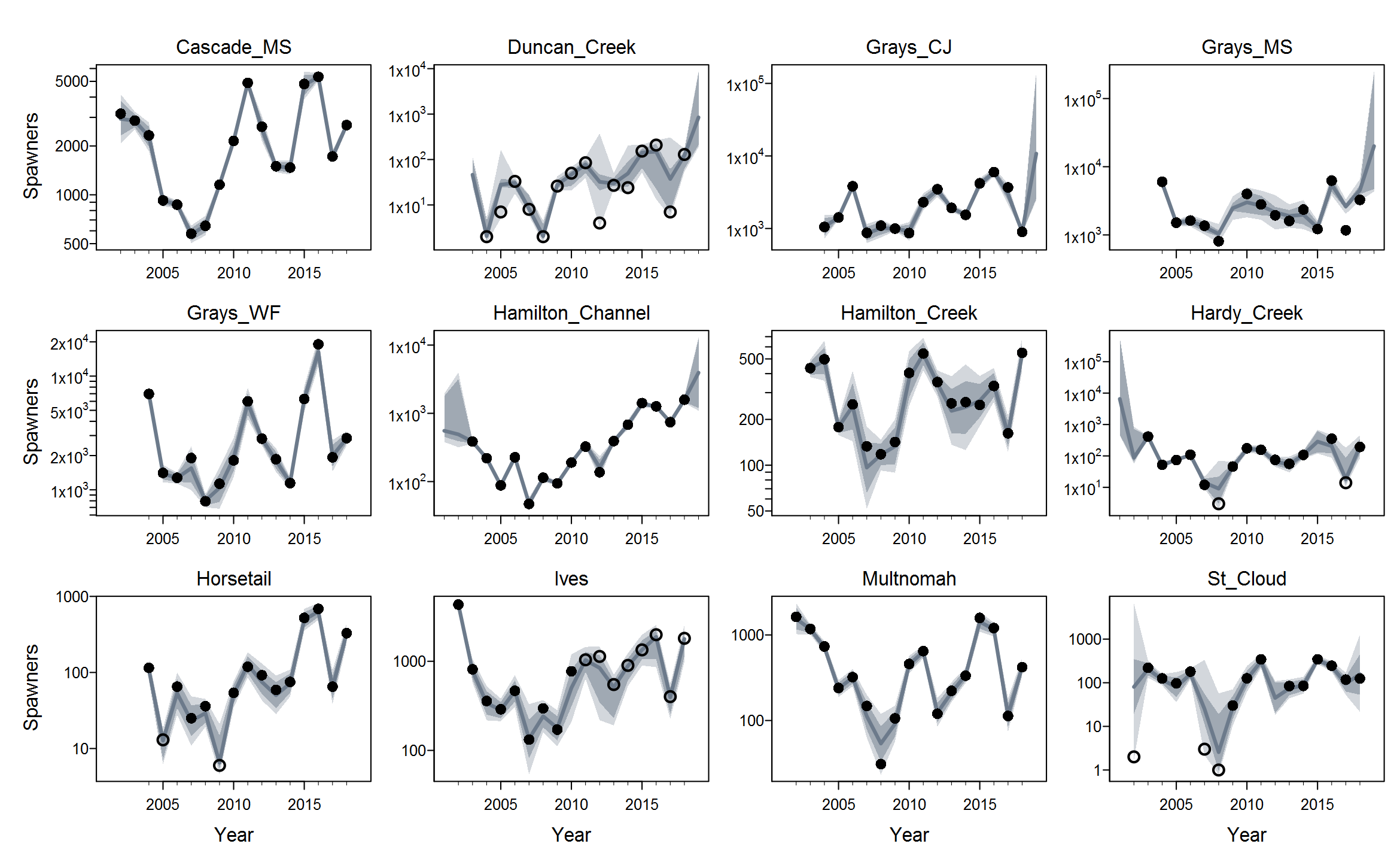
Rmaxunder the Ricker model. I'm not quite sure what's up with that, but I suspect that using population-specific estimates of spawning habitat (river km or ha) would improve things by making theRmaxrandom effects more exchangeable when expressed in units of density.The plots below show the fits from the Ricker model. Points are observed data, lines are posterior medians, and shading indicates the 95% credible interval of the states (dark) or the observations (light). Generally these look pretty good! Interestingly, the four populations in the
Gorge_MSgroup are much less synchronous than you might expect if they were really all highly connected or even quasi-panmictic. That could be one reason why the models struggled to fit the 8-population grouping.There is of course more due diligence needed for these fits, including more careful prior-posterior comparisons and formal model selection. Next I'd like to integrate the juvenile data and fit two-stage models. And then we can start customizing, perhaps starting with the sample-based observation error estimates.
Any questions / comments / suggestions so far?