Open eugeneyan opened 4 years ago
Hey Eugene, came across your great article from LinkedIn! Had a couple of discussion points/questions.
Using numpy.random.randint only takes 11 ms for me to generate 2 million integers, while a simplified version of your approach without shuffling took 34 ms for me (for the latter, I don't know if there's a faster way to do it). Experimental results attached.
https://uploads.disquscdn.c...
I'm also wondering how the negative items in the test set were generated in the end using your approach of consuming the array 2 elements at a time. Did you check for every pair (a,b) whether (a,b) was in the positive set (i.e. had a score of > 0.5), and then add it to the negative set if that was not true?
For the 'pure' MF without biases, it does seem a bit interesting to me that there is such a 'cliff of death' behavior and exactly at the 0.5 threshold too. Is this something you have observed in other problems before and/or do you have any intuition as to why this happens? I'm actually curious to replicate it to see what's going on.
The curves in the models with bias seem more in line with what I expected - is the only difference in the models that each item has a single bias parameter?
Thanks!
Comment by Daryl Lim on 2020-01-21T08:50:45Z
Hi Daryl,
For the sampling, there's a set of product IDs to sample from (e.g., B001T9NUFS, B003AVEU6, etc.) and not integers. That explains why it's slow as we have to example the set instead of just integer sampling with upper and lower bounds.
Yes, each negative-pair generated was checked to ensure that it was not the same as the positive-pair considered. I didn't not check for the entire positive set (and neither did the word2vec implementation).
This is pretty unusual to me too. Yes, the only difference is the additional bias embedding (dimension = 1). Would love to hear from your findings.
Comment by Eugene Yan on 2020-01-22T04:44:05Z
Hi Eugene, very interesting article, also the follow up! For this particular article I don't get what indeed you use as embedding, the string product IDs directly or their integer transformation, as the bullets points in Section "Implementation 1:..." suggest. I also wonder because to my knowledge Pytorch does not support string tensors.
Thanks for answering!
Comment by René Hommel on 2020-04-05T19:26:27Z
Thanks for this question René! To your question, a mapping between the string IDs and their integers is created and saved. It is the integers that are used as embedding keys in PyTorch.
Comment by Eugene Yan on 2020-04-05T21:58:32Z
Hi, Eugene! Please help me out here: I understood the nature of "Continuous labels" but I don't understand the objective you use for training and how we get from "Continuous labels" to ROC AUC calculations.
Hey Ilya,
TL;DR: While we use continuous labels for training, the output layer is a sigmoid that return scores from 0 - 1.
Why use continuous labels? Because they're able to better distinguish the strength of product-pair relationships. Here's a breakdown on binary vs. continuous labels.
Binary labels: A pair of products have a label of 1 if they have any, or multiple, relationships (e.g., also viewed
, also bought
, bought together
); zero otherwise.
This means that a pair of products which only have the also viewed
will have the same label as a pair of products which have all three relationships (i.e., also viewed
, also bought
, bought together
). While this approach can tell us if a pair of products have, or do not have, a relationship, it doesn't distinguish the strength of the relationship.
Continuous labels: To distinguish between the strengths of relationships, we use the following labels (instead of 1 or 0) - bought together
= 1.2, also bought
= 1.0, also viewed
= 0.5.
So, binary labels have values of 0 or 1.0, continuous labels have values of 0, 0.5, 1.0, 1,2.
Regardless of the type of label, we get predictions from a simple sigmoid, and predictions will range from 0 - 1. (See code for matrix factorization on binary labels and continuous labels). Nonetheless, we use binary cross entropy loss for binary labels, and mean square error loss for continuous labels.
Given that the final layer for both binary and continuous labels is a sigmoid, we can use ROC AUC for both.
Wow, such a comprehensive answer. ) First off, I'm very sorry that I overlooked the link to the repo 🤦 All is clear now. I got confused because, for me, regression and classification were like "two different worlds" due to projects I previously worked on. But I can see it makes sense here.
P.S. Probably it would be a good idea to incorporate your excellent comment into the article to help someone like me in the future
Thanks for the idea Ilya! Have added it into the article, right after the precision recall curves for Matrix Factorization (continuous labels).
Hi Eugene, Great article - really insightful.
Can you throw some more light on what exactly is cliff of death
and how the second model with bias is more production friendly even when it has lesser precision and recall?
Hi Eugene, thanks for sharing the project, I have learned a lot!
I have two questions:
IIUC you measure AUC-ROC for continuous label by getting the sigmoid predictions and then compare them against the binary versions of the val dataset right? So even though in training dataset our labels are continous, in val dataset we use binary labels so that we can measure AUC-ROC.
How does this approach fit in the Retrieval-Ranking phases of a RecSys? Is this a model in the retrieval phase? If yes then at inference step do we just retrieve candidate recommendations based on similarity-lookup on top of the learned embeddings?
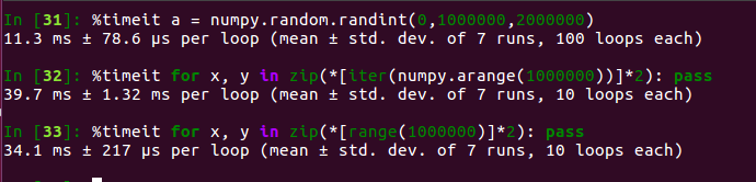
Migrated from json into utteranc.es