facebook / prophet

Tool for producing high quality forecasts for time series data that has multiple seasonality with linear or non-linear growth.
https://facebook.github.io/prophet
MIT License
18.46k stars 4.53k forks source link

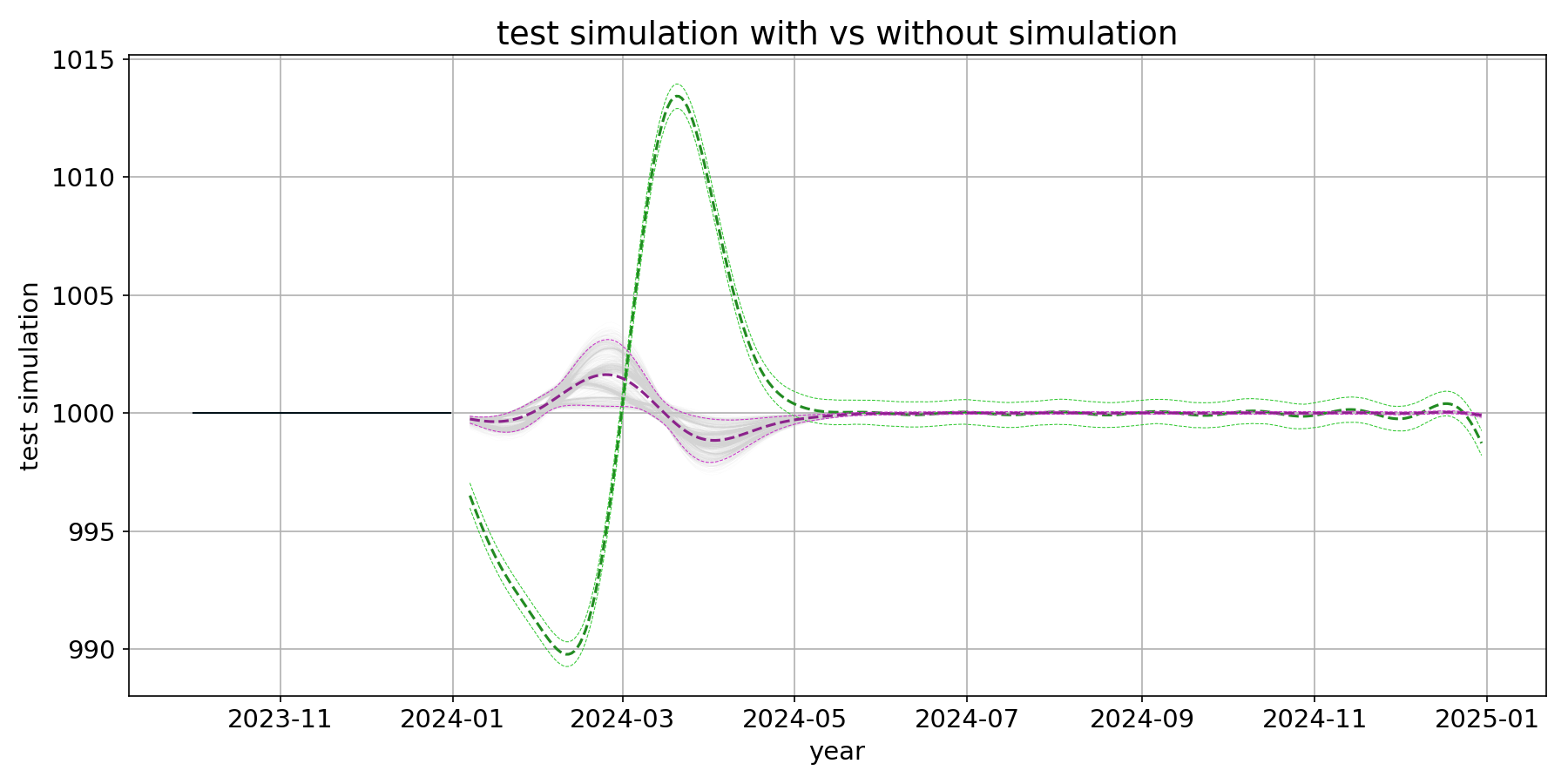
Forecast-Interval: MCMC simulation results are shifted compared to non-MCMC results #2415

Open KathyGCY opened 1 year ago

KathyGCY commented 1 year ago

Forecast-Interval: MCMC simulation results are shifted compared to non-MCMC results Here's a replicable code. Using prophet pip install --upgrade --force-reinstall --no-cache prophet==1.0.1

RESULTS:

Green ones are the Here's the demo data

Screenshot 2023-04-26 at 2 24 53 PM

Here's the results: download (1)

CODE:

Step 1 get the demo data

import numpy as np
import pandas as pd
import matplotlib.pyplot as plt

# Parameters
num_days = 365
growth_rate = 0.1
carrying_capacity = 1000
weekly_amplitude = 50

# Time indices
time_indices = np.arange(num_days)

# Logistic growth function
def logistic_growth(t, r, K):
    return K / (1 + (K - 1) * np.exp(-r * t))

# Weekly seasonality function
def weekly_seasonality(t, amplitude):
    return amplitude * np.sin(2 * np.pi * t / 7)

# Generate time series data
trend = logistic_growth(time_indices, growth_rate, carrying_capacity)
seasonality = weekly_seasonality(time_indices, weekly_amplitude)
time_series = trend + seasonality

# Create a DataFrame with dates and values
dates = pd.date_range(start='2023-01-01', periods=num_days, freq='D')
data = pd.DataFrame({'date': dates, 'value': time_series})
# Extend the DataFrame for 365 more days
additional_dates = pd.date_range(start='2024-01-01', periods=365, freq='D')
additional_data = pd.DataFrame({'date': additional_dates, 'value': np.nan})

# Concatenate the two DataFrames
data = pd.concat([data, additional_data], ignore_index=True)

# Plot the time series
plt.figure(figsize=(10, 6))
plt.plot(data['date'], data['value'], label='Logistic Trend with Weekly Seasonality')
plt.xlabel('date')
plt.ylabel('value')
plt.legend()
plt.show()
plt.savefig(f'demo data.png', dpi=150)

data['cap'] = 1000
data['floor'] = 0
data

Step 2, Get Prophet set up


from pandas import DataFrame
from prophet import Prophet
PROPHET_OPTIMIZATION_ITER = 500

def prophet_simulation(
    train: DataFrame,
    args: dict,
    hyperparams: dict
) -> DataFrame:
    train_ts_col = args["train_timestamp_col"]
    train_val_col = args["train_value_col"]
    cap_ts_col = args["cap_timestamp_col"]
    cap_val_col = args["cap_value_col"]
    floor_ts_col = args["floor_timestamp_col"]
    floor_val_col = args["floor_value_col"]
    reg_ts_col = args["reg_timestamp_col"]
    reg_val_cols = args["reg_value_col"]
    time_freq = args["time_freq"]

    cols = {train_ts_col: "ds", train_val_col: "y"}
    # create capacity if provided
    if cap_ts_col:
        cols[cap_val_col] = "cap"
        cap = train[[cap_ts_col, cap_val_col]]
        cap.rename(columns={cap_ts_col: "ds", cap_val_col: "cap"}, inplace=True)
    # create floor if provided
    if floor_ts_col:
        cols[floor_val_col] = "floor"
        floor = train[[floor_ts_col, floor_val_col]]
        floor.rename(
            columns={floor_ts_col: "ds", floor_val_col: "floor"}, inplace=True
        )
    # create regressors if provided
    if reg_ts_col:
        for reg_col in reg_val_cols:
            cols[reg_col] = reg_col
        reg = train[[reg_ts_col] + reg_val_cols]
        reg.rename(columns={reg_ts_col: "ds"}, inplace=True)
    ts = train[cols.keys()]
    last_ix = ts[train_val_col].last_valid_index()
    ts = ts[ts.index <= last_ix]
    ts.rename(columns=cols, inplace=True)

    # initialize prophet
    optimization_algo = hyperparams.pop("optimization_algo", None)
    optimization_iter = hyperparams.pop("optimization_iter", None)

    # by default we don't want Newton fallback because it's too slow
    # and makes the jobs stuck and fail in some cases
    # but this can always be overridden by user
    newton_fallback = hyperparams.pop("newton_fallback", False)
    hyperparams['interval_width'] = 0.9

    model = Prophet(**hyperparams)
    # add regressors if provided
    if reg_ts_col:
        for col in reg.columns.drop("ds"):
            model.add_regressor(
                col, prior_scale=None, standardize="auto", mode=None
            )

    # fit prophet
    model.stan_backend.set_options(newton_fallback=newton_fallback)
    kwargs = {}
    if optimization_algo:
        kwargs["algorithm"] = optimization_algo
    if optimization_iter:
        kwargs["iter"] = optimization_iter
    else:
        # by default, we cap the number of iterations to 500 to cater for
        # slow convergence, performance issues and job failures.
        # but this can always be overridden by user
        kwargs["iter"] = PROPHET_OPTIMIZATION_ITER
    model.fit(ts, **kwargs)
    # make data frame with future dates
    forecast_len = args["forecast_length"]
    future = model.make_future_dataframe(periods=forecast_len, freq=time_freq)
    # merge capacity if provided
    if cap_ts_col:
        future = future.merge(cap, how="left", on="ds")
    # merge floor if provided
    if floor_ts_col:
        future = future.merge(floor, how="left", on="ds")
    # merge regressors if provided
    if reg_ts_col:
        future = future.merge(reg, how="left", on="ds")

    # run forecast
    actual_forecast = model.predict(future)

    forecast = actual_forecast[
        ["ds", "yhat", "yhat_lower", "yhat_upper"]
    ]
    forecast = forecast.iloc[-forecast_len:]
    forecast["yhat"] = np.where(forecast["yhat"] < 0, 0, forecast["yhat"])
    forecast["yhat_lower"] = np.where(
        forecast["yhat_lower"] < 0,
        0,
        forecast["yhat_lower"],
    )
    forecast.rename(
        columns={
            "ds": train_ts_col,
            "yhat": train_val_col,
            "yhat_lower": f"{train_val_col}_lower",
            "yhat_upper": f"{train_val_col}_upper",
        },
        inplace=True,
    )
    if input_hp["mcmc_samples"] > 0:
        sim_predictive_samples = model.predictive_samples(future)
        df_simulated_yhat = pd.DataFrame(sim_predictive_samples['yhat']).iloc[-forecast_len:]
        df_simulated_trend = pd.DataFrame(sim_predictive_samples['trend']).iloc[-forecast_len:]
        df_simulated_yhat.columns = [f'S_yhat_{i:04d}' for i in range(1, 1001)]
        df_simulated_trend.columns = [f'S_tr_{i:04d}' for i in range(1, 1001)]
        return forecast, model, sim_predictive_samples, actual_forecast
    else:
        return forecast, model

Step 3, Hyperparam and Arguments

input_hp = {'changepoint_prior_scale': 0.05, 'changepoint_range': 0.8, 'growth': 'logistic', 'seasonality_mode': 'additive', 'seasonality_prior_scale': 0.01, 'yearly_seasonality': True}

input_arg = {'forecast_length': 365,
             'train_timestamp_col': "date",
             'train_value_col': "value",
             'reg_timestamp_col': None,
             'reg_value_col': None,
             "cap_timestamp_col": "date",
             "cap_value_col": "cap",
             "floor_timestamp_col": 'date',
             "floor_value_col": "floor",
             'time_freq': "d"}

Step 4, Run 2 versions, with and without MCMC

input_hp["mcmc_samples"] = 300
forecast_mcmc, model_mcmc, sim_predictive_samples, actual_forecast = prophet_simulation(
    train = data,
    args=input_arg,
    hyperparams = input_hp
)

input_hp["mcmc_samples"] = 0
forecast, model = prophet_simulation(
    train = data,
    args=input_arg,
    hyperparams = input_hp
)

Step 5, Compare output


df_simulated_yhat = pd.DataFrame(sim_predictive_samples['yhat']).iloc[-365:]
df_simulated_trend = pd.DataFrame(sim_predictive_samples['trend']).iloc[-365:]
df_simulated_yhat.columns = [f'S_yhat_{i:04d}' for i in range(1, 1001)]
df_simulated_trend.columns = [f'S_tr_{i:04d}' for i in range(1, 1001)]
df_out_act_ = data[['date', 'value']].dropna().reset_index(drop = True)
forecast_mcmc.columns = ['date', 'forecast_MCMC', 'lower_MCMC', 'upper_MCMC']
forecast.columns = ['date', 'forecast', 'lower', 'upper']
df_simulated_yhat['date'] = forecast_mcmc['date']
df_simulated_trend['date'] = forecast_mcmc['date']

# Actual-Forecast-Simulation (AFS)
df_afs = pd.merge(pd.merge(pd.merge(df_out_act_, 
                                    forecast, # forecast_mcmc
                                    on = 'date', 
                                    how = 'outer'),
                           forecast_mcmc, 
                           on = 'date', how = 'outer'
                          ),
                  df_simulated_yhat, 
                  on = 'date', how = 'outer'
                 )
df_afs

columns_to_plot = ['value', 'forecast', 'lower', 'upper', 'forecast_MCMC', 'lower_MCMC', 'upper_MCMC']
sim_columns_to_plot =  [f'S_yhat_{i:04d}' for i in range(1, 1001)]
df_one_country_ = df_afs
df_one_country_ = df_one_country_.rolling(7).apply(lambda x : np.nanmean(x))
df_one_country_['date'] = df_afs['date']
df_one_country_ = df_one_country_[df_one_country_['date'] >= '2023-10-01'].reset_index(drop = True)
plt.rcParams.update({'figure.figsize': (12, 6), 'figure.dpi': 150,
                    'axes.labelsize': 14,'axes.titlesize':18, 'legend.fontsize': 14, 'xtick.labelsize': 14, 'ytick.labelsize': 14})
fig, ax = plt.subplots()
for ser in sim_columns_to_plot + columns_to_plot:
    df_fil = df_one_country_[['date', ser]]
    lstyle = '-' if ('value' in ser) else '--'
    if ser in sim_columns_to_plot:
        this_colour = 'lightgrey'
        lstyle = "dotted"
        linewidth = 0.05
    elif ser == 'value':
        this_colour = '#001219'
        linewidth = 1
    elif ser == 'forecast':
        this_colour = '#228B22'
        linewidth = 1.5
    elif (ser == 'lower') | (ser == 'upper'):
        this_colour = '#31C831'
        linewidth = 0.5
    elif ser == 'forecast_MCMC':
        this_colour = '#8b228b'
        linewidth = 1.5
    elif (ser == 'lower_MCMC') | (ser == 'upper_MCMC'):
        this_colour = '#c831c8'
        linewidth = 0.5
    else:
        this_colour = '#D8D8D8'
        lstyle = "dotted"
        linewidth = 0.05
    ax.plot(df_fil['date'], df_fil[ser],
            label=ser, linewidth=linewidth, linestyle=lstyle, color = this_colour)
    ax.xaxis.label.set_size(14)
    ax.yaxis.label.set_size(14)

ax.set_ylabel('test simulation', fontsize=14)
ax.set_xlabel('year', fontsize=14)
# ax.legend(loc='upper left')
ax.grid()
ax.set_title('test simulation with vs without simulation')
fig.tight_layout()
fig.show()
plt.savefig(f'test simulation with vs without simulation.png', dpi=150)
plt.close()
``
KathyGCY commented 1 year ago

I have a theory. I did more testing and realized this is very unique to LOGISTIC trend. In fact if I simply switch to linear trend, the MCMC vs non-MCMC results are more aligned.

download (2)

QUESTION

Is this because when we MCMC, the cap / floor also participate in the simulation? Meaning that the cap for each simulated path might be slightly different? Would that explain the discrepancy?

FYI Here's the code for replication

New Step 1

import numpy as np
import pandas as pd
import matplotlib.pyplot as plt

# Parameters
num_days = 365
slope = 2
intercept = 100
weekly_amplitude = 50

# Time indices
time_indices = np.arange(num_days)

# Linear growth function
def linear_growth(t, m, b):
    return m * t + b

# Weekly seasonality function
def weekly_seasonality(t, amplitude):
    return amplitude * np.sin(2 * np.pi * t / 7)

# Generate time series data
trend = linear_growth(time_indices, slope, intercept)
seasonality = weekly_seasonality(time_indices, weekly_amplitude)
time_series = trend + seasonality

# Create a DataFrame with dates and values
dates = pd.date_range(start='2023-01-01', periods=num_days, freq='D')
data = pd.DataFrame({'date': dates, 'value': time_series})
# Extend the DataFrame for 365 more days
additional_dates = pd.date_range(start='2024-01-01', periods=365, freq='D')
additional_data = pd.DataFrame({'date': additional_dates, 'value': np.nan})

# Concatenate the two DataFrames
data = pd.concat([data, additional_data], ignore_index=True)

# Plot the time series
plt.figure(figsize=(10, 6))
plt.plot(data['date'], data['value'], label='Linear Trend with Weekly Seasonality')
plt.xlabel('date')
plt.ylabel('value')
plt.legend()
plt.show()

New Step 3

input_hp = {'changepoint_prior_scale': 0.05, 'changepoint_range': 0.8, 'growth': 'linear', 'seasonality_mode': 'additive', 'seasonality_prior_scale': 0.01, 'yearly_seasonality': True}

input_arg = {'forecast_length': 365,
             'train_timestamp_col': "date",
             'train_value_col': "value",
             'reg_timestamp_col': None,
             'reg_value_col': None,
             "cap_timestamp_col": None,
             "cap_value_col": None,
             "floor_timestamp_col": None,
             "floor_value_col": None,
             'time_freq': "d"}

And you run through step 4 and 5 exactly the same with no code change.