 Hamedloghmani
commented
1 year ago
Hamedloghmani
commented
1 year ago Thank you for the explanation @hosseinfani
Please read the description above @edwinpaul121 We can have a meeting about it if you think more explanation is required.
Open hosseinfani opened 1 year ago
Hamedloghmani
commented
1 year ago Thank you for the explanation @hosseinfani
Please read the description above @edwinpaul121 We can have a meeting about it if you think more explanation is required.
 edwinpaul121
commented
1 year ago
edwinpaul121
commented
1 year ago @Hamedloghmani, yes I'd like to have a meeting about this so I can get a better understanding of the task.
Hamedloghmani
commented
1 year ago @edwinpaul121 , sure. I'll get in touch in MS Teams and schedule a meeting soon.
edwinpaul121
commented
1 year ago Hi, I've gotten the 1st part of the problem done. Please verify and let me know if any changes need to be made.
import matplotlib.pyplot as plt
import statistics

def plot_distribution(data1,data2):
    '''
        @args
        float list for x axis values
        float list for y axis values
    '''
    # Calculations : mean, std dev, mean + 1 std dev, mean + 3 std dev
    mean = statistics.mean(data1)
    stdDev = statistics.stdev(data1)

    fig, ax = plt.subplots(figsize = (10,6))

    # Plots data
    ax.scatter(x = data1, y = data2)

    # Plotting vertical lines to indicate mean, mean + 1 * stdev and mean + 3 stdev
    ax.axvline(mean)
    ax.axvline(mean + stdDev)
    ax.axvline(mean + (3 * stdDev))

    # Titles for x and y axes
    plt.xlabel("X-Axis Values")
    plt.ylabel("Y-Axis Values")

    # Adding grid to display
    plt.grid()

    # Displays graph
    plt.show()
2 test cases for the above function :
x_vals = [1.2, 3.4, 5.6, 7.8, 9.0]
y_vals = [10.1, 8.9, 6.7, 4.5, 2.3]
xval = [0.695, 0.767, 1.058, 0.248, 0.381, 0.467, 0.2317]
yval = [0.126, 0.141, 0.247, 0.060, 0.083, 0.115, 0.0276]
Hamedloghmani
commented
1 year ago Hi @edwinpaul121
Thanks a lot for the implementation and progress report. I'll go over your code and example asap. Then we'll move on to the second part.
Thank you
edwinpaul121
commented
1 year ago Hi, here's an updated version of the code for the first part. Would we require an option to save the graph for this function as well? Changes made: Docstrings format +1 argument to indicate how many standard deviations to be plotted loop to plot required standard deviations
import matplotlib.pyplot as plt
import statistics

def plot_distribution(data1 : list, data2 : list, n : int):
    """
    Args:
        data1: Index of experts
        data2: Number of teams
        n: number of std dev to plot
    """
    # Calculations : mean, std dev, mean + 1 std dev, mean + 3 std dev
    mean = statistics.mean(data1)
    stdDev = statistics.stdev(data1)

    fig, ax = plt.subplots(figsize = (10, 6))

    # Plots data
    ax.scatter(x = data1, y = data2)

    # Plotting vertical line to indicate mean
    ax.axvline(mean)

    # Plotting vertical lines for mean + n * stdev
    for i in range(1, n + 1):
        ax.axvline(mean + i * stdDev)

    # Titles for x and y axes
    plt.xlabel("X-Axis Values")
    plt.ylabel("Y-Axis Values")

    # Adding grid to display
    plt.grid()

    # Displays graph
plt.show()Hello @edwinpaul121 Thanks a lot for the update. I'll go over your code today and let you know asap before the pull request.
Thanks
edwinpaul121
commented
1 year ago Hi, updating on some of the issues that I am facing right now,
1) The mid point of the data set is not being calculated properly
2) Moreover the issue does not require the mid point of the data set, rather the mid point that divides the area under the curve created by the data into two equal halves, which is also not being calculated properly. What I tried doing was finding the total area and dividing it into 2 halves but wasn't sure how to get the ending limit of the first half which I thought might get the point that divides the area into two equal halves.
3) Plotting of the mid point line is limited to mid value of data set and does not expand the range of the whole data set. Unless the interpolated x and y axis values are used. For example : 1.2, 3.4, 5.6, 7.8, 9.0 needs to have a mid value of (9.0 - 1.2) / 2 = 3.9 ~ 4 (technically not correct with regards to division of area as there are y-axis points as well, but this is with context to the x-axis alone) but it has a mid value (median) of 5.6 which is the middle most data in the set. The plotted value is the value stored at the index value indicating the mid point and not the actual mid point of the data set. This issue can be changed using interpolation but that comes with the same conditions as mentioned in the code where the data will not be plotted at exact values.
Here is the code with a few sample runs (The red lines show the interpolated plot) :
import matplotlib.pyplot as plt
import numpy as np
from scipy import interpolate

def area_under_curve(data_x : list, data_y : list):
    """
    Args:
        data1: Index of experts
        data2: # of teams

    """

    fig, ax = plt.subplots(figsize = (10,6))

    #------------------------------------------------------------------------------------------------------------------------------------------------
    # To plot a line graph of the data, interpolation can be used which creates a function based on the data points
    f = interpolate.interp1d(data_x, data_y, kind='linear')
    xnew = np.arange(min(data_x), max(data_x), 0.1) # returns evenly spaced values from the data set
    ynew = f(xnew)
    ax.plot(xnew, ynew, color = 'red')

    # the new x and y values could be used separately and we can continue with its own plot, however it does not show the exact values in the graph,
    #  rather just gives a good idea of how the data set can be interpreted
    #------------------------------------------------------------------------------------------------------------------------------------------------

    # Find the index of the midpoint of the curve
    total_area = np.trapz(data_y, data_x)
    half_area = total_area / 2
    cum_area = np.cumsum(data_y)
    mid_index = np.searchsorted(cum_area, half_area)
    #mid_index = len(data_x) // 2
    #mid_index = (max(data_x) - min(data_x)) // 2

    # Scatter plot of data
    ax.scatter(x = data_x, y = data_y)

    ax.plot(data_x, data_y, color = "green", alpha = 0.7) # Joins all points by a line

    # Fill left half of the area under the curve in blue
    ax.fill_between(data_x[ : mid_index + 1], data_y[ : mid_index + 1], color='blue', alpha=0.5)

    # Fill right half of the area under the curve in orange
    ax.fill_between(data_x[mid_index : ], data_y[mid_index : ], color='orange', alpha=0.5)

    # Titles for x and y axes
    plt.xlabel("X-Axis Values (Index of Experts)")
    plt.ylabel("Y-Axis Values (# Teams)")

    # Adding grid to display
    plt.grid()

    # Displays graph
    plt.show()
x_vals = [1.2, 3.4, 5.6, 7.8, 9.0]
y_vals = [10.1, 8.9, 6.7, 4.5, 2.3]xval = [0.695, 0.767, 1.058, 0.248, 0.381, 0.467, 0.2317]
yval = [0.126, 0.141, 0.247, 0.060, 0.083, 0.115, 0.0276]Hi @edwinpaul121 Thanks for sharing an update. I'll go over your issue and update this comment shortly. Thanks
edwinpaul121
commented
1 year ago @Hamedloghmani, just a follow up on that update, if the arange step value is changed to a value of 0.001, the graph becomes accurate so the plotted lines work well. This would be the line of code that changes
xnew = np.arange(min(data_x), max(data_x), 0.001)So that might be sorted but still working on the other issues. Thank you
edwinpaul121
commented
1 year ago Examples of how it looks now with the same data set. The mid point is just adjusted for now but isn't accurate still:
edwinpaul121
commented
1 year ago Hi @Hamedloghmani @hosseinfani, just got done working on all of the issues I mentioned earlier. I kind of brute forced finding the mid point that divides the area under the curve into 2 equal halves by creating a function that loops through the x axis values to find the exact middle by comparing the left and right areas rounded to 3 decimal points, so let me know if there's still a better and more efficient way of doing it.
But here's the final code, it includes 2 functions (one of them being a helper that calculates the midpoint, it can just be integrated as one function if required) :
import matplotlib.pyplot as plt
import numpy as np
from scipy import interpolate

def area_under_curve(data_x : list, data_y : list):
    """
    Args:
        data1: Index of experts
        data2: # of teams

    """

    fig, ax = plt.subplots(figsize = (10,6))

    # To plot a line graph of the data, interpolation can be used which creates a function based on the data points
    f = interpolate.interp1d(data_x, data_y, kind='linear')
    xnew = np.arange(min(data_x), max(data_x), 0.001) # returns evenly spaced values from the data set
    ynew = f(xnew)
    ax.plot(xnew, ynew, color = 'red')

    mid_index = midP_calc(xnew, ynew) # helper function that calculates the mid point of the data set that divides the area equally

    # Fill left half of the area under the curve in blue
    ax.fill_between(xnew[ : mid_index + 1], ynew[ : mid_index + 1], color='blue', alpha=0.5)

    # Fill right half of the area under the curve in orange
    ax.fill_between(xnew[mid_index : ], ynew[mid_index : ], color='orange', alpha=0.5)

    # Scatter plot of data
    ax.scatter(x = data_x, y = data_y)

    # Titles for x and y axes
    plt.xlabel("X-Axis Values (Index of Experts)")
    plt.ylabel("Y-Axis Values (# Teams)")

    # Adding grid to display
    plt.grid()

    # Displays graph
    plt.show()
This is the helper function :
def midP_calc(x : list, y : list):
    mid_index = len(x) // 2

    # Dividing the area under the curve into 2 halves
    left_area = np.trapz(y[ : mid_index + 1], x[ : mid_index + 1])
    right_area = np.trapz(y[mid_index : ], x[mid_index : ])

    # Finding the mid point that divides it equally
    while(left_area != right_area):
        if(left_area > right_area):
            mid_index -= 1
        else:
            mid_index += 1
        left_area = round(np.trapz(y[ : mid_index + 1], x[ : mid_index + 1]), 3)
        right_area = round(np.trapz(y[mid_index : ], x[mid_index : ]), 3)

    return mid_index
And here's the final output with the same axis values as mentioned earlier:
Hamedloghmani
commented
1 year ago Hi @edwinpaul121 , Thank you so much for the update. The results look nice. Please make a pull request with the code that you kindly wrote for the first and second parts of your task. I'll refactor and make minor changes afterwards. Thanks
edwinpaul121
commented
1 year ago Hi @Hamedloghmani, just got done refining the previous code a little bit. I've changed the helper function that calculates the mid point to binary search from linear so I think that should help with the run time a bit. I've done a few tests but I'm not sure how it might affect different systems with different configurations, in mine however there seems to be a noticeable decrease in run time. Here's the updated code :
import matplotlib.pyplot as plt
import numpy as np
from scipy import interpolate

def area_under_curve(data_x: list, data_y: list, xlabel: str, ylabel: str, lcolor='green', rcolor='orange'):
    """
    Args:
        data1: Index of experts
        data2: # of teams
        xlabel: label for x axis
        ylabel: label for y axis
    """

    fig, ax = plt.subplots(figsize = (10,6))

    # To plot a line graph of the data, interpolation can be used which creates a function based on the data points
    f = interpolate.interp1d(data_x, data_y, kind='linear')
    xnew = np.arange(min(data_x), max(data_x), 0.001) # returns evenly spaced values from the data set
    ynew = f(xnew)
    ax.plot(xnew, ynew, color = 'red')

    mid_index = mid_calc(xnew, ynew) # helper function that calculates the mid point of the data set that divides the area equally

    # Fill left half of the area under the curve in blue
    ax.fill_between(xnew[ : mid_index + 1], ynew[ : mid_index + 1], color=lcolor, alpha=0.3)

    # Fill right half of the area under the curve in orange
    ax.fill_between(xnew[mid_index : ], ynew[mid_index : ], color=rcolor, alpha=0.5)

    # Scatter plot of data
    ax.scatter(x = data_x, y = data_y)

    # Titles for x and y axes
    plt.xlabel(xlabel)
    plt.ylabel(ylabel)

    # Appearance settings
    ax.grid(True, color="#93a1a1", alpha=0.3)
    ax.minorticks_off()
    ax.xaxis.get_label().set_size(12)
    ax.yaxis.get_label().set_size(12)
    plt.legend(fontsize='small')
    ax.set_facecolor('whitesmoke')

    # Displays graph
    plt.show()
Along with the updated helper function :
def mid_calc(x : np.ndarray, y : np.ndarray)->int:
    """
    Helper function that calculates the middle point of the data set that divides the area equally
    Args:
        x: values of the x-axis
        y: values of the y-axis
    Returns:
        mid_index: index of the middle point
    """
    # Creating a start and end point for binary search
    start = 0
    end = len(x) - 1
    mid_index = (start + end) // 2

    # Dividing the area under the curve into 2 halves
    left_area = round(np.trapz(y[ : mid_index + 1], x[ : mid_index + 1]), 3)
    right_area = round(np.trapz(y[mid_index : ], x[mid_index : ]), 3)

    # Finding the middle point that divides it equally
    while(left_area != right_area and start <= end):

        if (left_area > right_area):
            end = mid_index
        elif (right_area > left_area):
            start = mid_index + 1
        else:
            return mid_index

        mid_index = (start + end) // 2

        left_area = round(np.trapz(y[ : mid_index + 1], x[ : mid_index + 1]), 3)
        right_area = round(np.trapz(y[mid_index : ], x[mid_index : ]), 3)

return mid_indexI've also updated the code to display mean and std. dev. to now show the mean with a dashed line:
import matplotlib.pyplot as plt
import statistics

def plot_distribution(data1 : list, data2 : list, n : int):
    """
    Args:
        data1: Index of experts
        data2: Number of teams
        n: number of std dev to plot
    """
    # Calculations : mean, std dev, mean + 1 std dev, mean + 3 std dev
    mean = statistics.mean(data1)
    stdDev = statistics.stdev(data1)

    fig, ax = plt.subplots(figsize = (10, 6))

    # Plots data
    ax.scatter(x = data1, y = data2)

    # Plotting vertical line to indicate mean
    ax.axvline(mean, linewidth = 1.5, linestyle = "--", color = 'red')

    # Plotting vertical lines for mean + n * stdev
    for i in range(1, n + 1):
        ax.axvline(mean + i * stdDev)

    # Titles for x and y axes
    plt.xlabel("X-Axis Values")
    plt.ylabel("Y-Axis Values")

    # Adding grid to display
    plt.grid()

    # Displays graph
plt.show()Hi @edwinpaul121 , thank you so much for the update. Please make a pull request and push these codes in the repo. I'll go over them and also test them over an actual dataset.
Thanks
edwinpaul121
commented
10 months ago Fixed a line in the mid_calc function that caused issues when running actual data through it. Had to change the comparison condition in the while loop as it lead to the code getting stuck. New comparison condition:
while(abs(left_area - right_area) > 0.05 and start <= end):
We need to justify the threshold of being popular vs. nonpopular based on distribution of experts. 1- We need a figure that shows the distribution and draw the lines on it to show the mean, mean+1std, mean+2std, ... with the value annotated on the lines. Something like this: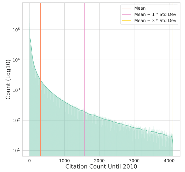
2- We need another figure that shows the area under the curve of distribution and split that area into two equal size, annotating each area with the same number. Something like this.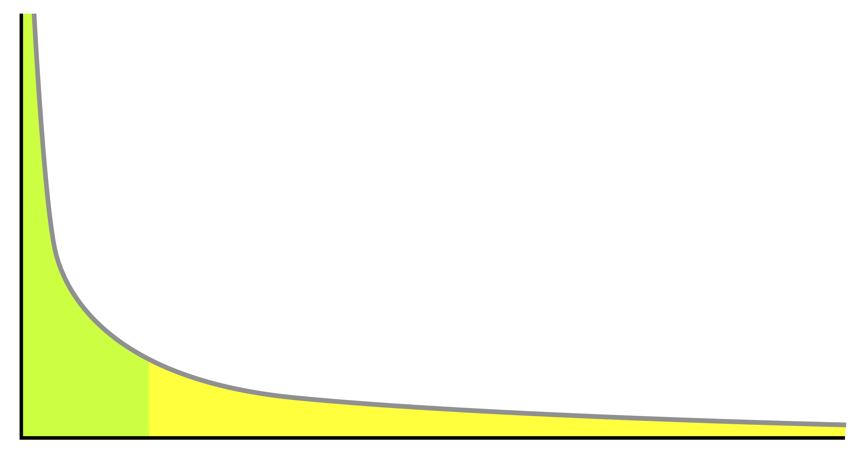
Hopefully, the mean and the area of splited under the carve are close.
@Hamedloghmani @edwinpaul121 How about this issue as the next task for Edwin?