Defining a 3D Plane Source

[CharlesDove]

I'm trying to define a plane source such that it outputs a plane wave, but I'm getting some odd-looking outputs. The following code seems to produce some pretty heavy fringes of some sort. Any thoughts? Ideally it would produce a smooth plane wave. Thanks!

import matplotlib.pyplot as plt

import fdtd
import fdtd.backend as bd
import numpy as np
import torch
import torch.autograd
import torch.nn
fdtd.set_backend("torch.cuda")

WAVELENGTH = 1550e-9
SPEED_LIGHT: float = 299_792_458.0  # [m/s] speed of light

grid = fdtd.Grid(
    (2.5e-5, 2.5e-5, 1.5e-5),
    # (161,161,97),
    grid_spacing=0.1 * WAVELENGTH,
    permittivity=1.0,
    permeability=1.0,
    # courant_number=0.3
)

grid[0, :, :] = fdtd.PeriodicBoundary(name="xbounds")
# grid[0:10, :, :] = fdtd.PML(name="pml_xlow")
# grid[-10:, :, :] = fdtd.PML(name="pml_xhigh")
grid[:, :, 0:10] = fdtd.PML(name="pml_zlow")
grid[:, :, -10:] = fdtd.PML(name="pml_zhigh")
grid[:, 0, :] = fdtd.PeriodicBoundary(name="ybounds")

grid[2:160,2:160,30:31] = fdtd.PlaneSource(
    period=WAVELENGTH / SPEED_LIGHT, name="linesource"
)
grid.run(300)
grid.visualize(z=80,show=True)

[flaport]

Hmm, I'm not sure what the intended behavior is supposed to be, but could it be that the light of the 'neighboring' cells (remember: you're using periodic boundaries) is starting to interfere with the light in the current cell? Look for example at the light at timestep 90 (grid.run(90)):

This looks like a proper source to me (admittedly, not exactly what I would expect from a PlaneSource, I will have to look into that).

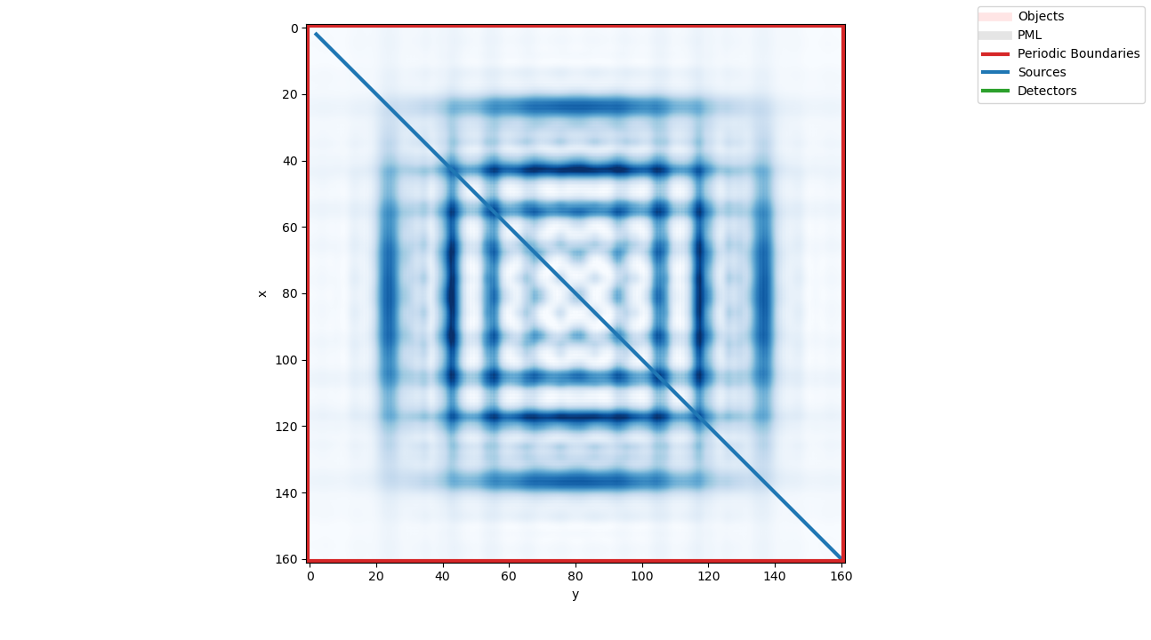
However, at timestep 100 (grid.run(100)) we see that the fringes because of interference with the light of neighboring cells start to appear:

To prevent these fringes, use PMLs everywhere:

grid[0:10, :, :] = fdtd.PML(name="pml_xlow")
grid[-10:, :, :] = fdtd.PML(name="pml_xhigh")
grid[:, 0:10, :] = fdtd.PML(name="pml_ylow")
grid[:, -10:, :] = fdtd.PML(name="pml_yhigh")
grid[:, :, 0:10] = fdtd.PML(name="pml_zlow")
grid[:, :, -10:] = fdtd.PML(name="pml_zhigh")

After 100 timesteps:

That said, you'll still see artifacts after 300 timesteps because the PML is never perfect and in practice you'll always have reflections at the PML:

To reduce those artifacts, increase the simulation area and the thickness of the PML:

As you can see, the fringes never completely go away, likely because of the naive PML implementation. If someone wants to attempt to implement a better PML, be my guest ;-)

[CharlesDove]

Hi @flaport, thanks for the thorough response and help! Hmm, using PML makes sense, but that plane wave indeed doesn't look quite right. For comparison, here's a plane wave from MEEP https://meep.readthedocs.io/en/latest/

import meep as mp
import matplotlib.pyplot as plt

pml_layers = [mp.PML(thickness=1)]
cell_size = mp.Vector3(10,10,10)

sources = [mp.Source(mp.ContinuousSource(1,is_integrated=True),
                     center=mp.Vector3(-4),
                     size=mp.Vector3(0,10,10),
                     component=mp.Ez)]

sim = mp.Simulation(resolution=10,
                    cell_size=cell_size,
                    boundary_layers=pml_layers,
                    sources=sources,
                    k_point=mp.Vector3())

sim.run(until=30)

sim.plot2D(fields=mp.Ez,
           output_plane=mp.Volume(center=mp.Vector3(),size=mp.Vector3(10,0,10)))
# plt.show()
plt.savefig('pw_side.png',bbox_inches='tight')
sim.plot2D(fields=mp.Ez,
           output_plane=mp.Volume(center=mp.Vector3(),size=mp.Vector3(0,10,10)))
plt.savefig('pw_front.png',bbox_inches='tight')

Any ideas what the cause might be?

[CharlesDove]

Actually the cause of this looks to be that the PlaneSource (also LineSource) is actually Gaussian and not uniform! Defined starting around line 402 in sources.py. Making that profile variable an array of ones doesn't immediately appear to make a functional plane wave for me, however. Also a uniform flat plane wave should (I think) be usable with periodic boundary conditions on its sides. EDIT: I suspect that an additional edit must be made in the PlaneSource's update_E function. Any thoughts?

[CharlesDove]

Figured it out. A plane source at z=N outputs the wrong polarization, which doesn't propagate. Changing it to something transverse solves the problem. Also there should probably be GaussianPlaneSource and UniformPlaneSource methods to reduce ambiguity. For line sources as well. I'll see if I can knock together a PR. :)

[flaport]

Hey Charles,

I'm happy you figured it out! a PR for this would be amazing, thanks 🙂

[flaport]

@CharlesDove , If you have the time, would you be willing to create a PR with your fix?