Best reproducible map competition for GISRUK 2019

Robinlovelace commented 5 years ago

Entries are welcome for 'best reproducible map' and 'most creative map'. This competition coincides with the GISRUK 2019 conference and at least 1 of the prizes will go to attendees of the R course we are teaching there based on the book.

Deadline for submissions: 10:30, British Summer Time (aka BST or UTC+1)

Criteria for 'best map'

Reproducible and based on well-written code
Use of aesthetics to ensure clear communication of the underlying data
Tells a story with the data that is relevant to policy, scientific or public debate

Criteria for 'most creative map'

Creative use of R to show geographic data in a new way
Unusual location or topic shown
Catches the attention

Please paste your entries here, as with the previous competition #371

rcatlord commented 5 years ago

Hi Robin - here's my entry to the 'best reproducible map' competition. The R code retrieves and plots allotments from OpenStreetMap for your chosen Local Authority.

library(sf) ; library(osmdata) ; library(tidyverse) ; library(tmap)
#> Linking to GEOS 3.6.1, GDAL 2.1.3, PROJ 4.9.3
#> Data (c) OpenStreetMap contributors, ODbL 1.0. http://www.openstreetmap.org/copyright
#> Warning: package 'tibble' was built under R version 3.5.2
#> Warning: package 'tidyr' was built under R version 3.5.2
#> Warning: package 'purrr' was built under R version 3.5.2
#> Warning: package 'dplyr' was built under R version 3.5.2
#> Warning: package 'stringr' was built under R version 3.5.2
#> Warning: package 'tmap' was built under R version 3.5.2
lad <- URLencode("Manchester")
boundary <- st_read(paste0("https://ons-inspire.esriuk.com/arcgis/rest/services/Administrative_Boundaries/Local_Authority_Districts_April_2019_Boundaries_UK_BGC/MapServer/0/query?where=lad19nm%20=%20%27", lad, "%27&outFields=lad19cd,lad19nm,long,lat&outSR=4326&f=geojson"))
#> Reading layer `OGRGeoJSON' from data source `https://ons-inspire.esriuk.com/arcgis/rest/services/Administrative_Boundaries/Local_Authority_Districts_April_2019_Boundaries_UK_BGC/MapServer/0/query?where=lad19nm%20=%20%27Manchester%27&outFields=lad19cd,lad19nm,long,lat&outSR=4326&f=geojson' using driver `GeoJSON'
#> Simple feature collection with 1 feature and 4 fields
#> geometry type:  POLYGON
#> dimension:      XY
#> bbox:           xmin: -2.319919 ymin: 53.34012 xmax: -2.146828 ymax: 53.54461
#> epsg (SRID):    4326
#> proj4string:    +proj=longlat +datum=WGS84 +no_defs
coords <- st_bbox(boundary) %>% as.vector()
osm <- opq(bbox = coords) %>%
  add_osm_feature(key = "landuse", value = "allotments") %>%
  osmdata_sf()
osm_polygons <- osm$osm_polygons
names(osm_polygons$geometry) <- NULL
feature <- osm_polygons %>% 
  st_transform(st_crs(boundary)) %>% 
  st_intersection(., boundary) 
#> although coordinates are longitude/latitude, st_intersection assumes that they are planar
#> Warning: attribute variables are assumed to be spatially constant
#> throughout all geometries
tmap_mode("view")
#> tmap mode set to interactive viewing
tm_shape(boundary) +
  tm_fill(
    col = "#DDDDCC", 
    alpha = 0.5,
    popup.vars = c("Name" = "lad19nm")
  ) +
  tm_borders() +
  tm_shape(feature) +
  tm_fill(
    col = "#7cfc00",
    popup.vars = c("Name" = "name")
  ) +
  tm_borders() +
  tm_layout(title = paste0("Allotments in ", lad)) +
  tm_basemap(server = "Esri.WorldGrayCanvas", alpha = 0.5)

^{Created on 2019-04-18 by the reprex package (v0.2.1)}

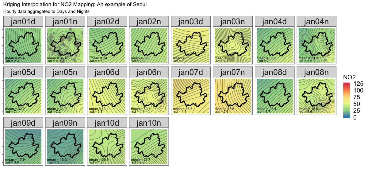
dataandcrowd commented 5 years ago

Hi Robin!

I didn't have enough time to run reprex, however, it seems to work fine. Note that the Kriging iteration takes around 5 minutes.

A space-time Kriging Interpolation for Seoul's NO2 Mapping

options(scipen = 100) # To see long decimal points
memory.size() # for WindowsOS
memory.limit(99999) # for WindowsOS

library(tidyverse)
library(sf)
library(raster)
library(rgdal)
library(automap)
library(gridExtra)

# set working directory so I know where the .zip file will be located
getwd()
#setwd(dir = "/some/path/")

# on the GitHub repository of interest
download.file(url = "https://github.com/mrsensible/GISRUK2019/archive/master.zip", 
              destfile = "GISRUK2019-master.zip")

# unzip the .zip file
unzip(zipfile = "GISRUK2019-master.zip")

# examine the contents
list.files('./GISRUK2019-master')
list.files('./GISRUK2019-master/data')

# Set Working Directory
setwd('./GISRUK2019-master')

# Load NO2 Pollution data
load("data/no2_jan.RData")

# Import moritoring stations from Seoul
stations <- read_sf("data/stations_10km.shp")
stations_df <- stations %>% st_set_geometry(NULL)

# Import Seoul Shapefile
seoul <- read_sf("data/Seoul_City.shp") %>% as('Spatial') %>% fortify()

no2.winter <- merge(no2.win.12hr, stations_df, by.x = c("Station.ID", "X", "Y"), by.y = c("Station", "X", "Y"))
coordinates(no2.winter) <- ~X+Y
proj4string(no2.winter) <- CRS("+init=epsg:5181")

#--Put Multiple Plots on a Single Page in R with spplot--##
plots <- lapply(names(no2.winter)[3:22], function(.x) spplot(no2.winter,.x))
do.call(grid.arrange,plots)

#################################################################
#--Generate auto Semivariograms in need to create Kriging maps--#
#################################################################
myList <- list()

for(i in 1:20) { 
  myList[[length(myList)+1]] <- autofitVariogram(no2.winter[[i+2]] ~ 1, no2.winter)
}
semvar <- lapply(myList, function(x) plot(x))
do.call(grid.arrange, semvar[1:4])

### Create gridcells for interpolation
seoul_grid <- data.frame(expand.grid(X = seq(min(no2.winter$X), max(no2.winter$X), length=200),
                                     Y = seq(min(no2.winter$Y), max(no2.winter$Y), length=200)))
coordinates(seoul_grid) <- ~X+Y
proj4string(seoul_grid) <- CRS("+init=epsg:5181") #Korean Central Belt 2000

##############
#--Kriging--##
##############
sum.squares <- vector()
var.model <- data.frame()
pred.model <- seoul_grid@coords

# This iteration takes 5 minutes!!

for(i in 1:20) {
  kriging_new <- autoKrige(no2.winter@data[,i+2]~ X + Y,
                           nmax = 20000,
                           input_data = no2.winter, 
                           new_data = seoul_grid)
  sum.squares <- append(sum.squares, kriging_new$sserr)
  kriging_new$var_model <- data.frame(y=i,kriging_new$var_model)
  var.model <- rbind(var.model, kriging_new$var_model)
  xyz <- as.data.frame(kriging_new$krige_output)
  p <- data.frame(xyz[,'var1.pred'])
  colnames(p) <- colnames(no2.winter@data)[i+2]
  pred.model <- cbind(pred.model, p)
} 

##-- Add ColNames
colnames(pred.model) <- c("X", "Y", "jan01d", "jan01n", "jan02d", "jan02n","jan03d", "jan03n", "jan04d", "jan04n", "jan05d", "jan05n", "jan06d", "jan06n", "jan07d", "jan07n", "jan08d", "jan08n", "jan09d", "jan09n", "jan10d", "jan10n")

##-- Mean and variance to display on map
stat <- pred.model %>% dplyr::select(-c(X,Y)) %>% 
        gather(factor_key = T) %>% 
        group_by(key) %>% summarise(mean= round(mean(value),1), sd= round(sd(value),1), 
                                    max = max(value),min = min(value)) %>% 
        rename(Hour = key)

##############################################
##-- Final Map: Kriging Interpolation map --##
##############################################

ras.krige.df <- pred.model %>% 
  reshape2::melt(id = c("X", "Y"), variable.name = "Hour", value.name = "NO2") 

ras.krige.df %>% 
  ggplot() +
  geom_tile(aes(x = X, y = Y, fill = NO2)) +
  scale_fill_distiller(palette = "Spectral", na.value = NA, limits = c(0,125), breaks = c(0,25,50,75,100,125)) +
  geom_contour(aes(x = X, y = Y, z = NO2),bins = 20, colour = "grey40", alpha = 0.7) +
  geom_path(data = seoul, aes(x = long, y = lat), color = 'black', size = 1) +
  geom_text(data = stat, aes(x = 187000,  y = 434000, label = paste0("mean = " , mean)), size = 3) + 
  geom_text(data = stat, aes(x = 184000,  y = 430500, label = paste0("sd = " , sd)), size = 3) + 
  labs(title = "Kriging Interpolation for NO2 Mapping: An example of Seoul", 
       subtitle = "Hourly data aggregated to Days and Nights (µg/m3)") +
  facet_wrap(~ Hour, ncol = 8) +
  theme_bw() +
  theme(axis.title.x=element_blank(),
        axis.text.x=element_blank(),
        axis.ticks.x=element_blank(),
        axis.text.y=element_blank(),
        axis.title.y=element_blank(),
        strip.text.x = element_text(size = 20),
        legend.title=element_text(size=15), 
        legend.text=element_text(size=15)                                  
  ) -> final # 1200 x 550 

# Export PNG
png("no2_seoul.png", width=1200, height=550, res=100)
final
dev.off()

# RMSE
RMSE <- function(observed, predicted) {
  sqrt(mean((predicted - observed)^2, na.rm=TRUE))}

for (i in 3:length(pred.model)){
  RMSE(mean(pred.model[, i]), pred.model[, i]) %>% print()
}

# convert to Raster Bricks
krige <- rasterFromXYZ(pred.model, 
                       crs="+proj=tmerc +lat_0=38 +lon_0=127 +k=1 +x_0=200000 +y_0=500000 +ellps=GRS80 +towgs84=0,0,0,0,0,0,0 +units=m +no_defs",
                       digits=5)

# Write Raster
writeRaster(krige, filename="seoul_no2_multilayer.tif", options="INTERLEAVE=BAND", overwrite=TRUE)

Rplot

Hyesop Shin, Dept.of Geography, University of Cambridge

agila5 commented 5 years ago

Hi! This is my submission for the map competition. I tried to represent a bivariate choropleth map for census data in Milan using tmap and following this blog post. This is the code.

# load packages
library(tidyverse)
library(magrittr)
library(sf)
library(tmap)

# download and unzip geodata and census data
temp_file_1 <- tempfile()
temp_file_2 <- tempfile()

download.file("http://www.istat.it/storage/cartografia/basi_territoriali/WGS_84_UTM/2011/R03_11_WGS84.zip", temp_file_1)
download.file("http://www.istat.it/storage/cartografia/variabili-censuarie/dati-cpa_2011.zip", temp_file_2)

unzip(temp_file_1)
unzip(temp_file_2)
unlink(temp_file_1)
unlink(temp_file_2)

# load geodata and census data
milan_census_geodata <- read_sf("R03_11_WGS84/R03_11_WGS84.shp") %>%
  filter(COD_ISTAT == 3015146) %>%
  mutate(SEZ2011 = as.character(SEZ2011))

milan_census_data <- read_delim(
  file = "Sezioni di Censimento/R03_indicatori_2011_sezioni.csv",
  delim = ";",
  escape_double = FALSE,
  col_types = cols(CODASC = col_integer(), SEZ2011 = col_character()),
  trim_ws = TRUE
) %>% 
  filter(CODPRO == 15, CODCOM == 146) %>% 
  select(SEZ2011, P1, E1)

milan_census_geodata is a sf containing geometries for all census areas in Milan while milan_census_data is a tibble containing the observed values for several variables. I decided to focus on two variables: P1 (total population) and E1 (total number of buildings).

# I want to focus on P1 (Population) and E1 (Buildings)
quantiles_P1 <- milan_census_data %>% 
  pull(P1) %>% 
  quantile(probs = seq(0, 1, length.out = 4))
quantiles_E1 <- milan_census_data %>% 
  pull(E1) %>% 
  quantile(probs = seq(0, 1, length.out = 4))

bivariate_color_scale <- tibble(
  "3 - 3" = "#3F2949", # high population and a lot of buildings
  "2 - 3" = "#435786",
  "1 - 3" = "#4885C1", # low populations and a lot of buildings (industrial area)
  "3 - 2" = "#77324C",
  "2 - 2" = "#806A8A", 
  "1 - 2" = "#89A1C8",
  "3 - 1" = "#AE3A4E", # high population and a few buildings (residential area)
  "2 - 1" = "#BC7C8F",
  "1 - 1" = "#CABED0", # rural or abandoned areas, parks, touristic locations (e.g. Duomo) or shopping district (e.g. City Life)
) %>%
  gather("group", "fill")

milan_census_data %<>% 
  mutate(
    P1_quantiles = cut(
      P1, 
      breaks = quantiles_P1, 
      include.lowest = TRUE
    ), 
    E1_quantiles = cut(
      E1, 
      breaks = quantiles_E1, 
      include.lowest = TRUE
    ), 
    group = paste(
      as.numeric(P1_quantiles), "-",
      as.numeric(E1_quantiles)
    )
  ) %>% 
  left_join(bivariate_color_scale, by = "group")

# Join the two datasets according to the ID variable

milan_join_geodata <- left_join(
  milan_census_geodata,
  milan_census_data,
  by = "SEZ2011"
) %>% 
  mutate_at(vars(P1, E1), replace_na, replace = 0) %>% 
  select(SEZ2011, P1, E1, group, fill)

Now I have to create the grid for the col value. First of all I created a rectangle whose height and width are equal to 15% of xrange and yrange of the municipality's bbox, then I copied the same rectangle 8 times. I set an offset between the first rectangle and the margins of the plot equal to 15% of the axis range.

# Create the grid
milan_bbox <- st_bbox(milan_census_geodata)
step_x <- (milan_bbox[3] - milan_bbox[1]) / 15
step_y <- (milan_bbox[4] - milan_bbox[2]) / 15

# Create the first rectangle
first_rectangle <- c(
  milan_bbox[1] + 1 * step_x, milan_bbox[2] + 1 * step_y, 
  milan_bbox[1] + 2 * step_x, milan_bbox[2] + 1 * step_y, 
  milan_bbox[1] + 2 * step_x, milan_bbox[2] + 2 * step_y, 
  milan_bbox[1] + 1 * step_x, milan_bbox[2] + 2 * step_y,
  milan_bbox[1] + 1 * step_x, milan_bbox[2] + 1 * step_y
)

# Copy it 8 times
list_of_rectangles <- list(
  first_rectangle + c(0 * step_x, 0 * step_y), 
  first_rectangle + c(1 * step_x, 0 * step_y), 
  first_rectangle + c(2 * step_x, 0 * step_y), 
  first_rectangle + c(0 * step_x, 1 * step_y), 
  first_rectangle + c(1 * step_x, 1 * step_y), 
  first_rectangle + c(2 * step_x, 1 * step_y), 
  first_rectangle + c(0 * step_x, 2 * step_y), 
  first_rectangle + c(1 * step_x, 2 * step_y), 
  first_rectangle + c(2 * step_x, 2 * step_y)
)

# Transform it as a list of polygons
geo_rectangles <- map(map(list_of_rectangles, ~ list(matrix(data = .x, ncol = 2, byrow = TRUE))), st_polygon)

# Create the sf
sf_rectangles <- st_sf(
  tibble(
    fill = c(
      "#CABED0", 
      "#89A1C8",
      "#4885C1", 
      "#BC7C8F",
      "#806A8A",
      "#435786",
      "#AE3A4E", 
      "#77324C",
      "#3F2949" 
    )
  ),
  geometry = geo_rectangles %>% st_sfc(), 
  crs = 32632
)

I had to revert the order of the colors since I'm creating the list of polygons from the left to the right of the plot and from the bottom to the top while the other tibble specifies the colors from top-right to bottom-left. This is the result.

tm_shape(milan_join_geodata) + 
  tm_polygons("fill") + 
  tm_shape(sf_rectangles) + 
  tm_polygons(col = "fill") + 
  tm_scale_bar(position = c("right", "bottom"), width = 0.15) + 
  tm_layout(
    main.title = "Bivariate choropleth map for Milan Census data."
  )

immagine

White values correspond to missing areas, red values correspond to industrial areas, light blue values correspond to residential areas and purple values to high populated areas with a lot of buildings. Grey areas correspond to rural and abandoned areas or touristic location (e.g. Duomo) and shopping ares (e.g. City Life).

I think that this example could be generalized and be somewhat related to this issue.

kchastko commented 5 years ago

Hi Robin,

Here is my bivariate choropleth map showing the relationship between tornado events and the proportion of people living in mobile homes in each county of the contiguous united states.


library(sf)
library(spData)
library(biscale)
library(ggplot2)
library(cowplot)

# Download tornado and mobile homw data from NOAA
download.file(url = "https://www.spc.noaa.gov/gis/svrgis/zipped/mobile_home_percentage_county.zip",
              destfile = "tornado.zip")

unzip(zipfile = "tornado.zip")
mHomes = st_read(dsn = "mobile_home_percentage_county.shp")

download.file(url = "https://www.spc.noaa.gov/gis/svrgis/zipped/1950-2017-torn-initpoint.zip",
              destfile = "tornado.zip")
unzip(zipfile = "tornado.zip")
tornadoes = st_read(dsn = "1950-2017-torn-initpoint/1950-2017-torn-initpoint.shp")

# Project all the data to albers equal area projection
tornadoes <- st_transform(tornadoes, 2163)
mHomes <- st_transform(mHomes, 2163)
us_states_proj <- st_transform(us_states, 2163)

# "Clip" data to the the contiguous united states
mHomes <- mHomes[us_states_proj, ]
tornadoes2 = tornadoes[us_states_proj, ]

# Find the count of tornadoes in each us county
torn_count = aggregate(tornadoes2, mHomes, length)
t_combined = cbind(mHomes, count = torn_count$mag)

# Set counties with no tornadoes to 0 (from defult NA)
t_combined$count[is.na(t_combined$count)] <- 0

#Create bivariate classification from proportion mobile homes
# and tornado count
data <- bi_class(t_combined, x = MobileHome, y = count) 

#Assign color palette
data <- bi_pal(data, pal = "DkBlue")

# Map the data using ggplot2
map <- ggplot() +
  geom_sf(data = data, aes(fill = bs_fill), color = "white", size = 0.1) +
  scale_fill_identity() +
  labs(
    title = "Tornado Events and Mobile Homes in the United States",
    subtitle = "Dark Blue (DkBlue) Palette"
  ) +
  bi_theme()
map

# Create the legend
bs <- bi_legend(pal = "DkBlue")

# draw legend
legend <- ggplot() +
  geom_tile(data = bs, mapping = aes(x = x, y = y, fill = bs_fill)) +
  scale_fill_identity() +
  labs(x = expression(paste("Higher Proportion Mobile Homes ", ""%->%"")),
       y = expression(paste("Higher Tornado Count ", ""%->%""))) +
  bi_theme() +
  theme(axis.title = element_text(size = 8)) +
  coord_fixed()

# combine map with legend
finalPlot <- ggdraw() +
  draw_plot(map, 0, 0, 1, 1) +
  draw_plot(legend, 0.0, 0.0, 0.3, 0.3)

# print map
finalPlot

# Save map as png
ggsave("finalPlot.png", width = 10, height = 7, units = "in")

finalPlot

Robinlovelace commented 5 years ago

Many thanks for your submissions @rcatlord, @mrsensible, @agila5 and @kchastko. We are really impressed by all the submissions, many thanks for showing that useful and beautiful maps can be reproducible!

Results coming soon.

Robinlovelace commented 5 years ago

Test for reproducibility from @rcatlord on my laptop gets a :heavy_check_mark:

library(sf) ; library(osmdata) ; library(tidyverse) ; library(tmap)
#> Linking to GEOS 3.7.0, GDAL 2.4.0, PROJ 5.2.0
#> Data (c) OpenStreetMap contributors, ODbL 1.0. http://www.openstreetmap.org/copyright
#> Linking to GEOS 3.6.1, GDAL 2.1.3, PROJ 4.9.3
#> Data (c) OpenStreetMap contributors, ODbL 1.0. http://www.openstreetmap.org/copyright
#> Warning: package 'tibble' was built under R version 3.5.2
#> Warning: package 'tidyr' was built under R version 3.5.2
#> Warning: package 'purrr' was built under R version 3.5.2
#> Warning: package 'dplyr' was built under R version 3.5.2
#> Warning: package 'stringr' was built under R version 3.5.2
#> Warning: package 'tmap' was built under R version 3.5.2
lad <- URLencode("Manchester")
boundary <- st_read(paste0("https://ons-inspire.esriuk.com/arcgis/rest/services/Administrative_Boundaries/Local_Authority_Districts_April_2019_Boundaries_UK_BGC/MapServer/0/query?where=lad19nm%20=%20%27", lad, "%27&outFields=lad19cd,lad19nm,long,lat&outSR=4326&f=geojson"))
#> Reading layer `OGRGeoJSON' from data source `https://ons-inspire.esriuk.com/arcgis/rest/services/Administrative_Boundaries/Local_Authority_Districts_April_2019_Boundaries_UK_BGC/MapServer/0/query?where=lad19nm%20=%20%27Manchester%27&outFields=lad19cd,lad19nm,long,lat&outSR=4326&f=geojson' using driver `GeoJSON'
#> Simple feature collection with 1 feature and 4 fields
#> geometry type:  POLYGON
#> dimension:      XY
#> bbox:           xmin: -2.319919 ymin: 53.34012 xmax: -2.146828 ymax: 53.54461
#> epsg (SRID):    4326
#> proj4string:    +proj=longlat +datum=WGS84 +no_defs
#> Reading layer `OGRGeoJSON' from data source `https://ons-inspire.esriuk.com/arcgis/rest/services/Administrative_Boundaries/Local_Authority_Districts_April_2019_Boundaries_UK_BGC/MapServer/0/query?where=lad19nm%20=%20%27Manchester%27&outFields=lad19cd,lad19nm,long,lat&outSR=4326&f=geojson' using driver `GeoJSON'
#> Simple feature collection with 1 feature and 4 fields
#> geometry type:  POLYGON
#> dimension:      XY
#> bbox:           xmin: -2.319919 ymin: 53.34012 xmax: -2.146828 ymax: 53.54461
#> epsg (SRID):    4326
#> proj4string:    +proj=longlat +datum=WGS84 +no_defs
coords <- st_bbox(boundary) %>% as.vector()
osm <- opq(bbox = coords) %>%
  add_osm_feature(key = "landuse", value = "allotments") %>%
  osmdata_sf()
osm_polygons <- osm$osm_polygons
names(osm_polygons$geometry) <- NULL
feature <- osm_polygons %>% 
  st_transform(st_crs(boundary)) %>% 
  st_intersection(., boundary) 
#> although coordinates are longitude/latitude, st_intersection assumes that they are planar
#> Warning: attribute variables are assumed to be spatially constant
#> throughout all geometries
#> although coordinates are longitude/latitude, st_intersection assumes that they are planar
#> Warning: attribute variables are assumed to be spatially constant
#> throughout all geometries
tmap_mode("view")
#> tmap mode set to interactive viewing
#> tmap mode set to interactive viewing
tm_shape(boundary) +
  tm_fill(
    col = "#DDDDCC", 
    alpha = 0.5,
    popup.vars = c("Name" = "lad19nm")
  ) +
  tm_borders() +
  tm_shape(feature) +
  tm_fill(
    col = "#7cfc00",
    popup.vars = c("Name" = "name")
  ) +
  tm_borders() +
  tm_layout(title = paste0("Allotments in ", lad)) +
  tm_basemap(server = "Esri.WorldGrayCanvas", alpha = 0.5)

^{Created on 2019-04-24 by the reprex package (v0.2.1)}

Robinlovelace commented 5 years ago

@mrsensible I could reproduce most of your map but had some issues on the robinlovelace/geocompr docker image:

options(scipen = 100) # To see long decimal points
> memory.size() # for WindowsOS
[1] Inf
Warning message:
'memory.size()' is Windows-specific 
> memory.limit(99999) # for WindowsOS
[1] Inf
Warning message:
'memory.limit()' is Windows-specific 
> 
> library(tidyverse)
> library(sf)
> library(raster)
> library(rgdal)
> library(automap)
> library(gridExtra)
> 
> 
> # set working directory so I know where the .zip file will be located
> getwd()
[1] "/home/rstudio/data/npct/pct-shiny"
> #setwd(dir = "/some/path/")
> 
> # on the GitHub repository of interest
> download.file(url = "https://github.com/mrsensible/GISRUK2019/archive/master.zip",
+               destfile = "GISRUK2019-master.zip")
trying URL 'https://github.com/mrsensible/GISRUK2019/archive/master.zip'
downloaded 167 KB

> 
> # unzip the .zip file
> unzip(zipfile = "GISRUK2019-master.zip")
> 
> # examine the contents
> list.files('./GISRUK2019-master')
[1] "data"             "GISRUK2019.Rproj" "LICENSE"          "no2_kriging.R"   
> list.files('./GISRUK2019-master/data')
 [1] "no2_jan.RData"      "road_10km_re.tif"   "Seoul_City.cpg"    
 [4] "Seoul_City.dbf"     "Seoul_City.prj"     "Seoul_City.shp"    
 [7] "Seoul_City.shp.xml" "Seoul_City.shx"     "stations_10km.dbf" 
[10] "stations_10km.prj"  "stations_10km.qpj"  "stations_10km.shp" 
[13] "stations_10km.shx" 
> 
> # Set Workding Directory
> setwd('./GISRUK2019-master')
> 
> 
> # Load NO2 Pollution data
> load("data/no2_jan.RData")
> 
> # Import moritoring stations from Seoul
> stations <- read_sf("data/stations_10km.shp")
> stations_df <- stations %>% st_set_geometry(NULL)
> 
> # Import Seoul Shapefile
> seoul <- read_sf("data/Seoul_City.shp") %>% as('Spatial') %>% fortify()
Regions defined for each Polygons
> 
> no2.winter <- merge(no2.win.12hr, stations_df, by.x = c("Station.ID", "X", "Y"), by.y = c("Station", "X", "Y"))
> coordinates(no2.winter) <- ~X+Y
> proj4string(no2.winter) <- CRS("+init=epsg:5181")
> 
> 
> #--Put Multiple Plots on a Single Page in R with spplot--##
> plots <- lapply(names(no2.winter)[3:22], function(.x) spplot(no2.winter,.x))
> do.call(grid.arrange,plots)
> 
> 
> #################################################################
> #--Generate auto Semivariograms in need to create Kriging maps--#
> #################################################################
> myList <- list()
> 
> for(i in 1:20) {
+   myList[[length(myList)+1]] <- autofitVariogram(no2.winter[[i+2]] ~ 1, no2.winter)
+ }
> semvar <- lapply(myList, function(x) plot(x))
> do.call(grid.arrange, semvar[1:4])
> 
> 
> ### Create gridcells for interpolation
> seoul_grid <- data.frame(expand.grid(X = seq(min(no2.winter$X), max(no2.winter$X), length=200),
+                                      Y = seq(min(no2.winter$Y), max(no2.winter$Y), length=200)))
> coordinates(seoul_grid) <- ~X+Y
> proj4string(seoul_grid) <- CRS("+init=epsg:5181") #Korean Central Belt 2000
> 
> 
> ##############
> #--Kriging--##
> ##############
> sum.squares <- vector()
> var.model <- data.frame()
> pred.model <- seoul_grid@coords
> 
> 
> # This iteration takes 5 minutes!!
> 
> for(i in 1:20) {
+   kriging_new <- autoKrige(no2.winter@data[,i+2]~ X + Y,
+                            nmax = 20000,
+                            input_data = no2.winter,
+                            new_data = seoul_grid)
+   sum.squares <- append(sum.squares, kriging_new$sserr)
+   kriging_new$var_model <- data.frame(y=i,kriging_new$var_model)
+   var.model <- rbind(var.model, kriging_new$var_model)
+   xyz <- as.data.frame(kriging_new$krige_output)
+   p <- data.frame(xyz[,'var1.pred'])
+   colnames(p) <- colnames(no2.winter@data)[i+2]
+   pred.model <- cbind(pred.model, p)
+ }
[using universal kriging]
Error in predict.gstat(g, newdata = newdata, block = block, nsim = nsim,  : 
  value not allowed for: Getest(): mode not specified
> 
> ##-- Add ColNames
> colnames(pred.model) <- c("X", "Y", "jan01d", "jan01n", "jan02d", "jan02n","jan03d", "jan03n", "jan04d", "jan04n", "jan05d", "jan05n", "jan06d", "jan06n", "jan07d", "jan07n", "jan08d", "jan08n", "jan09d", "jan09n", "jan10d", "jan10n")
Error in dimnames(x) <- dn : 
  length of 'dimnames' [2] not equal to array extent
> 
> 
> ##-- Mean and variance to display on map
> stat <- pred.model %>% dplyr::select(-c(X,Y)) %>%
+   gather(factor_key = T) %>%
+   group_by(key) %>% summarise(mean= round(mean(value),1), sd= round(sd(value),1),
+                               max = max(value),min = min(value)) %>%
+   rename(Hour = key)
Error in UseMethod("select_") : 
  no applicable method for 'select_' applied to an object of class "c('matrix', 'double', 'numeric')"
> 
> ##############################################
> ##-- Final Map: Kriging Interpolation map --##
> ##############################################
> 
> ras.krige.df <- pred.model %>%
+   reshape2::melt(id = c("X", "Y"), variable.name = "Hour", value.name = "NO2")
> 
> ras.krige.df %>%
+   ggplot() +
+   geom_tile(aes(x = X, y = Y, fill = NO2)) +
+   scale_fill_distiller(palette = "Spectral", na.value = NA, limits = c(0,125), breaks = c(0,25,50,75,100,125)) +
+   geom_contour(aes(x = X, y = Y, z = NO2),bins = 20, colour = "grey40", alpha = 0.7) +
+   scale_color_gradientn(limits = c(100,300), colours=c("orangered", "firebrick")) +
+   geom_path(data = seoul, aes(x = long, y = lat), color = 'black', size = 1) +
+   geom_text(data = stat, aes(x = 187000,  y = 434000, label = paste0("mean = " , mean)), size = 3) +
+   geom_text(data = stat, aes(x = 184000,  y = 430500, label = paste0("sd = " , sd)), size = 3) +
+   labs(title = "Kriging Interpolation for NO2 Mapping: An example of Seoul",
+        subtitle = "Hourly data aggregated to Days and Nights") +
+   facet_wrap(~ Hour, ncol = 8) +
+   theme_bw() +
+   theme(axis.title.x=element_blank(),
+         axis.text.x=element_blank(),
+         axis.ticks.x=element_blank(),
+         axis.text.y=element_blank(),
+         axis.title.y=element_blank(),
+         strip.text.x = element_text(size = 20),
+         legend.title=element_text(size=15),
+         legend.text=element_text(size=15)
+   ) # 1200 x 550
Error: At least one layer must contain all faceting variables: `Hour`.
* Plot is missing `Hour`
* Layer 1 is missing `Hour`
* Layer 2 is missing `Hour`
* Layer 3 is missing `Hour`
* Layer 4 is missing `Hour`
* Layer 5 is missing `Hour`
> 
> 
> # RMSE
> 
> RMSE <- function(observed, predicted) {
+   sqrt(mean((predicted - observed)^2, na.rm=TRUE))}
> 
> for (i in 3:length(pred.model)){
+   RMSE(mean(pred.model[, i]), pred.model[, i]) %>% print()
+ }
Error in pred.model[, i] : subscript out of bounds
> 
> 
> # convert to Raster Bricks
> krige <- rasterFromXYZ(pred.model,
+                        crs="+proj=tmerc +lat_0=38 +lon_0=127 +k=1 +x_0=200000 +y_0=500000 +ellps=GRS80 +towgs84=0,0,0,0,0,0,0 +units=m +no_defs",
+                        digits=5)
> 
> # Write Raster
> writeRaster(krige, filename="seoul_no2_multilayer.tif", options="INTERLEAVE=BAND", overwrite=TRUE)
Warning message:
In .local(x, filename, ...) : all cell values are NA
> magick::image_read("seoul_no2_multilayer.tif")
Error in magick_image_readpath(path, density, depth, strip) : 
  Magick: Sorry, can not handle images with 32-bit samples. `/home/rstudio/data/npct/pct-shiny/GISRUK2019-master/seoul_no2_multilayer.tif' @ error/tiff.c/TIFFErrors/564
> webshot::webshot("seoul_no2_multilayer.tif")
PhantomJS not found. You can install it with webshot::install_phantomjs(). If it is installed, please make sure the phantomjs executable can be found via the PATH variable.
NULL
> browseURL("seoul_no2_multilayer.tif")
> list.files()
[1] "data"                     "GISRUK2019.Rproj"         "LICENSE"                 
[4] "no2_kriging.R"            "seoul_no2_multilayer.tif"
> ras.krige.df %>%
+   ggplot() +
+   geom_tile(aes(x = X, y = Y, fill = NO2)) +
+   scale_fill_distiller(palette = "Spectral", na.value = NA, limits = c(0,125), breaks = c(0,25,50,75,100,125)) +
+   geom_contour(aes(x = X, y = Y, z = NO2),bins = 20, colour = "grey40", alpha = 0.7) +
+   scale_color_gradientn(limits = c(100,300), colours=c("orangered", "firebrick")) +
+   geom_path(data = seoul, aes(x = long, y = lat), color = 'black', size = 1) +
+   geom_text(data = stat, aes(x = 187000,  y = 434000, label = paste0("mean = " , mean)), size = 3) +
+   geom_text(data = stat, aes(x = 184000,  y = 430500, label = paste0("sd = " , sd)), size = 3) +
+   labs(title = "Kriging Interpolation for NO2 Mapping: An example of Seoul",
+        subtitle = "Hourly data aggregated to Days and Nights") +
+   facet_wrap(~ Hour, ncol = 8) +
+   theme_bw() +
+   theme(axis.title.x=element_blank(),
+         axis.text.x=element_blank(),
+         axis.ticks.x=element_blank(),
+         axis.text.y=element_blank(),
+         axis.title.y=element_blank(),
+         strip.text.x = element_text(size = 20),
+         legend.title=element_text(size=15),
+         legend.text=element_text(size=15)
+   ) # 1200 x 550
Error: At least one layer must contain all faceting variables: `Hour`.
* Plot is missing `Hour`
* Layer 1 is missing `Hour`
* Layer 2 is missing `Hour`
* Layer 3 is missing `Hour`
* Layer 4 is missing `Hour`
* Layer 5 is missing `Hour`

Robinlovelace commented 5 years ago

@agila5 I could fully reproduce your map after downloading MB of data ; ) great work, as illustrated below:

dataandcrowd commented 5 years ago

@mrsensible I could reproduce most of your map but had some issues on the robinlovelace/geocompr docker image:

Are you using Linux or MacOSX? If so, you might have problems installing the gstat package. Although the package asks you to install version 2.0, you have to say no and install the older version if you are not running Windows. Can I kindly ask you to have another try?

Robinlovelace commented 5 years ago

@kchastko after installing the new biscales package I could reproduce it as follows:

remotes::install_github("slu-openGIS/biscale")
#> Skipping install of 'biscale' from a github remote, the SHA1 (9b72073b) has not changed since last install.
#>   Use `force = TRUE` to force installation

library(sf)
#> Linking to GEOS 3.7.0, GDAL 2.4.0, PROJ 5.2.0
library(spData)
library(biscale)
library(ggplot2)
library(cowplot)
#> 
#> Attaching package: 'cowplot'
#> The following object is masked from 'package:ggplot2':
#> 
#>     ggsave

# Download tornado and mobile homw data from NOAA
download.file(url = "https://www.spc.noaa.gov/gis/svrgis/zipped/mobile_home_percentage_county.zip",
              destfile = "tornado.zip")

unzip(zipfile = "tornado.zip")
mHomes = st_read(dsn = "mobile_home_percentage_county.shp")
#> Reading layer `mobile_home_percentage_county' from data source `/tmp/RtmpvlMhXj/reprex274717383dc8/mobile_home_percentage_county.shp' using driver `ESRI Shapefile'
#> replacing null geometries with empty geometries
#> Simple feature collection with 3238 features and 10 fields (with 38 geometries empty)
#> geometry type:  GEOMETRY
#> dimension:      XY
#> bbox:           xmin: -2350004 ymin: -1875700 xmax: 3466149 ymax: 2431662
#> epsg (SRID):    102004
#> proj4string:    +proj=lcc +lat_1=33 +lat_2=45 +lat_0=39 +lon_0=-96 +x_0=0 +y_0=0 +datum=NAD83 +units=m +no_defs

download.file(url = "https://www.spc.noaa.gov/gis/svrgis/zipped/1950-2017-torn-initpoint.zip",
              destfile = "tornado.zip")
unzip(zipfile = "tornado.zip")
tornadoes = st_read(dsn = "1950-2017-torn-initpoint/1950-2017-torn-initpoint.shp")
#> Reading layer `1950-2017-torn-initpoint' from data source `/tmp/RtmpvlMhXj/reprex274717383dc8/1950-2017-torn-initpoint/1950-2017-torn-initpoint.shp' using driver `ESRI Shapefile'
#> Simple feature collection with 62519 features and 22 fields
#> geometry type:  POINT
#> dimension:      XY
#> bbox:           xmin: -163.53 ymin: 18.13 xmax: -64.9 ymax: 61.02
#> epsg (SRID):    4326
#> proj4string:    +proj=longlat +datum=WGS84 +no_defs

# Project all the data to albers equal area projection
tornadoes <- st_transform(tornadoes, 2163)
mHomes <- st_transform(mHomes, 2163)
us_states_proj <- st_transform(us_states, 2163)

# "Clip" data to the the contiguous united states
mHomes <- mHomes[us_states_proj, ]
tornadoes2 = tornadoes[us_states_proj, ]

# Find the count of tornadoes in each us county
torn_count = aggregate(tornadoes2, mHomes, length)
t_combined = cbind(mHomes, count = torn_count$mag)

# Set counties with no tornadoes to 0 (from defult NA)
t_combined$count[is.na(t_combined$count)] <- 0

#Create bivariate classification from proportion mobile homes
# and tornado count
data <- bi_class(t_combined, x = MobileHome, y = count) 

#Assign color palette
data <- bi_pal(data, pal = "DkBlue")

# Map the data using ggplot2
map <- ggplot() +
  geom_sf(data = data, aes(fill = bs_fill), color = "white", size = 0.1) +
  scale_fill_identity() +
  labs(
    title = "Tornado Events and Mobile Homes in the United States",
    subtitle = "Dark Blue (DkBlue) Palette"
  ) +
  bi_theme()
map


# Create the legend
bs <- bi_legend(pal = "DkBlue")

# draw legend
legend <- ggplot() +
  geom_tile(data = bs, mapping = aes(x = x, y = y, fill = bs_fill)) +
  scale_fill_identity() +
  labs(x = expression(paste("Higher Proportion Mobile Homes ", ""%->%"")),
       y = expression(paste("Higher Tornado Count ", ""%->%""))) +
  bi_theme() +
  theme(axis.title = element_text(size = 8)) +
  coord_fixed()

# combine map with legend
finalPlot <- ggdraw() +
  draw_plot(map, 0, 0, 1, 1) +
  draw_plot(legend, 0.0, 0.0, 0.3, 0.3)

# print map
finalPlot


# Save map as png
ggsave("finalPlot.png", width = 10, height = 7, units = "in")

^{Created on 2019-04-24 by the reprex package (v0.2.1)}

Robinlovelace commented 5 years ago

Impressed at all these entries, thanks again for creative and certainly useful maps.

Unfortunately there can only be 2 winners, however, and these go @mrsensible (who received a copy of the book locally) and @agila5.

Reasoning below, in reverse order:

@kchastko your map is beautiful, reproducible and highly relevant politically. Unfortunately it was submitted just after the deadline of 10:30 BST.
@agila5 your map should much work going into the data preparation and download side, and innovative use of tmap to generate a bivariate colourscheme. Congratulations!
@mrsensible your map is well-thought and communicates a huge amount of space in relatively little space. Yours shows creative use of facets and novel pre-processing so wins the most creative map (in addition to being the only 'local' submission ; )
@rcatlord the generalisability and simplicity of this map are great strengths. Many thanks for an excellent map, showing something that could genuinely be useful for people interested in land ownership and sustainable food.

Any feedback welcome. @mrsensible your code is still running on my laptop and making its fan spin!

Robinlovelace commented 5 years ago

Update: @mrsensible you are right, it eventually ran on my computer and generated this result:

Robinlovelace commented 5 years ago

Output below...

^{Created on 2019-04-24 by the reprex package (v0.2.1)}

Session info

``` r devtools::session_info() #> ─ Session info ────────────────────────────────────────────────────────── #> setting value #> version R version 3.5.3 (2019-03-11) #> os Ubuntu 18.04.2 LTS #> system x86_64, linux-gnu #> ui X11 #> language en_GB:en #> collate en_GB.UTF-8 #> ctype en_GB.UTF-8 #> tz Europe/London #> date 2019-04-24 #> #> ─ Packages ────────────────────────────────────────────────────────────── #> package * version date lib source #> assertthat 0.2.1 2019-03-21 [1] CRAN (R 3.5.3) #> backports 1.1.4 2019-04-10 [3] CRAN (R 3.5.3) #> callr 3.2.0 2019-03-15 [1] CRAN (R 3.5.3) #> cli 1.1.0 2019-03-19 [1] CRAN (R 3.5.3) #> crayon 1.3.4 2017-09-16 [3] CRAN (R 3.5.0) #> desc 1.2.0 2018-05-01 [3] CRAN (R 3.5.0) #> devtools 2.0.2 2019-04-08 [1] CRAN (R 3.5.3) #> digest 0.6.18 2018-10-10 [3] CRAN (R 3.5.1) #> evaluate 0.13 2019-02-12 [3] CRAN (R 3.5.2) #> fs 1.2.7 2019-03-19 [1] CRAN (R 3.5.3) #> glue 1.3.1 2019-03-12 [1] CRAN (R 3.5.3) #> highr 0.8 2019-03-20 [1] CRAN (R 3.5.3) #> htmltools 0.3.6 2017-04-28 [3] CRAN (R 3.5.0) #> knitr 1.22 2019-03-08 [1] CRAN (R 3.5.2) #> magrittr 1.5 2014-11-22 [3] CRAN (R 3.5.0) #> memoise 1.1.0 2017-04-21 [3] CRAN (R 3.5.0) #> pkgbuild 1.0.3 2019-03-20 [1] CRAN (R 3.5.3) #> pkgload 1.0.2 2018-10-29 [3] CRAN (R 3.5.1) #> prettyunits 1.0.2 2015-07-13 [1] CRAN (R 3.5.1) #> processx 3.3.0 2019-03-10 [1] CRAN (R 3.5.3) #> ps 1.3.0 2018-12-21 [3] CRAN (R 3.5.2) #> R6 2.4.0 2019-02-14 [1] CRAN (R 3.5.2) #> Rcpp 1.0.1 2019-03-17 [1] CRAN (R 3.5.3) #> remotes 2.0.4 2019-04-10 [1] CRAN (R 3.5.3) #> rlang 0.3.4 2019-04-07 [1] CRAN (R 3.5.3) #> rmarkdown 1.12 2019-03-14 [1] CRAN (R 3.5.3) #> rprojroot 1.3-2 2018-01-03 [1] CRAN (R 3.5.1) #> sessioninfo 1.1.1 2018-11-05 [1] CRAN (R 3.5.1) #> stringi 1.4.3 2019-03-12 [1] CRAN (R 3.5.3) #> stringr 1.4.0 2019-02-10 [1] CRAN (R 3.5.2) #> testthat 2.0.1 2018-10-13 [1] CRAN (R 3.5.1) #> usethis 1.5.0 2019-04-07 [1] CRAN (R 3.5.3) #> withr 2.1.2 2018-03-15 [3] CRAN (R 3.5.0) #> xfun 0.6 2019-04-02 [1] CRAN (R 3.5.3) #> yaml 2.2.0 2018-07-25 [3] CRAN (R 3.5.1) #> #> [1] /home/robin/R/x86_64-pc-linux-gnu-library/3.5 #> [2] /usr/local/lib/R/site-library #> [3] /usr/lib/R/site-library #> [4] /usr/lib/R/library ``` options(scipen = 100) # To see long decimal points > memory.size() # for WindowsOS [1] Inf Warning message: 'memory.size()' is Windows-specific > memory.limit(99999) # for WindowsOS [1] Inf Warning message: 'memory.limit()' is Windows-specific > > library(tidyverse) ── Attaching packages ────────────────────────────────────────────────── tidyverse 1.2.1 ── ✔ ggplot2 3.1.1 ✔ purrr 0.3.2 ✔ tibble 2.1.1 ✔ dplyr 0.8.0.1 ✔ tidyr 0.8.3 ✔ stringr 1.4.0 ✔ readr 1.3.1 ✔ forcats 0.4.0 ── Conflicts ───────────────────────────────────────────────────── tidyverse_conflicts() ── ✖ dplyr::filter() masks stats::filter() ✖ dplyr::lag() masks stats::lag() > library(sf) Linking to GEOS 3.7.0, GDAL 2.4.0, PROJ 5.2.0 > library(raster) Loading required package: sp Attaching package: ‘raster’ The following object is masked from ‘package:dplyr’: select The following object is masked from ‘package:tidyr’: extract > library(rgdal) rgdal: version: 1.4-3, (SVN revision 828) Geospatial Data Abstraction Library extensions to R successfully loaded Loaded GDAL runtime: GDAL 2.4.0, released 2018/12/14 Path to GDAL shared files: /usr/share/gdal GDAL binary built with GEOS: TRUE Loaded PROJ.4 runtime: Rel. 5.2.0, September 15th, 2018, [PJ_VERSION: 520] Path to PROJ.4 shared files: (autodetected) Linking to sp version: 1.3-1 > library(automap) > library(gridExtra) Attaching package: ‘gridExtra’ The following object is masked from ‘package:dplyr’: combine > > > # set working directory so I know where the .zip file will be located > getwd() [1] "/home/robin/geocompr/geocompkg" > #setwd(dir = "/some/path/") > > # on the GitHub repository of interest > download.file(url = "https://github.com/mrsensible/GISRUK2019/archive/master.zip", + destfile = "GISRUK2019-master.zip") trying URL 'https://github.com/mrsensible/GISRUK2019/archive/master.zip' downloaded 167 KB > > # unzip the .zip file > unzip(zipfile = "GISRUK2019-master.zip") > > # examine the contents > list.files('./GISRUK2019-master') [1] "data" "GISRUK2019.Rproj" "LICENSE" "no2_kriging.R" > list.files('./GISRUK2019-master/data') [1] "no2_jan.RData" "road_10km_re.tif" "Seoul_City.cpg" "Seoul_City.dbf" [5] "Seoul_City.prj" "Seoul_City.shp" "Seoul_City.shp.xml" "Seoul_City.shx" [9] "stations_10km.dbf" "stations_10km.prj" "stations_10km.qpj" "stations_10km.shp" [13] "stations_10km.shx" > > # Set Workding Directory > setwd('./GISRUK2019-master') > > > # Load NO2 Pollution data > load("data/no2_jan.RData") > > # Import moritoring stations from Seoul > stations <- read_sf("data/stations_10km.shp") > stations_df <- stations %>% st_set_geometry(NULL) > > # Import Seoul Shapefile > seoul <- read_sf("data/Seoul_City.shp") %>% as('Spatial') %>% fortify() Regions defined for each Polygons > > no2.winter <- merge(no2.win.12hr, stations_df, by.x = c("Station.ID", "X", "Y"), by.y = c("Station", "X", "Y")) > coordinates(no2.winter) <- ~X+Y > proj4string(no2.winter) <- CRS("+init=epsg:5181") > > > #--Put Multiple Plots on a Single Page in R with spplot--## > plots <- lapply(names(no2.winter)[3:22], function(.x) spplot(no2.winter,.x)) > do.call(grid.arrange,plots) > > > ################################################################# > #--Generate auto Semivariograms in need to create Kriging maps--# > ################################################################# > myList <- list() > > for(i in 1:20) { + myList[[length(myList)+1]] <- autofitVariogram(no2.winter[[i+2]] ~ 1, no2.winter) + } > semvar <- lapply(myList, function(x) plot(x)) > do.call(grid.arrange, semvar[1:4]) > > > ### Create gridcells for interpolation > seoul_grid <- data.frame(expand.grid(X = seq(min(no2.winter$X), max(no2.winter$X), length=200), + Y = seq(min(no2.winter$Y), max(no2.winter$Y), length=200))) > coordinates(seoul_grid) <- ~X+Y > proj4string(seoul_grid) <- CRS("+init=epsg:5181") #Korean Central Belt 2000 > > > ############## > #--Kriging--## > ############## > sum.squares <- vector() > var.model <- data.frame() > pred.model <- seoul_grid@coords > > > # This iteration takes 5 minutes!! > > for(i in 1:20) { + kriging_new <- autoKrige(no2.winter@data[,i+2]~ X + Y, + nmax = 20000, + input_data = no2.winter, + new_data = seoul_grid) + sum.squares <- append(sum.squares, kriging_new$sserr) + kriging_new$var_model <- data.frame(y=i,kriging_new$var_model) + var.model <- rbind(var.model, kriging_new$var_model) + xyz <- as.data.frame(kriging_new$krige_output) + p <- data.frame(xyz[,'var1.pred']) + colnames(p) <- colnames(no2.winter@data)[i+2] + pred.model <- cbind(pred.model, p) + } [using universal kriging] [using universal kriging] [using universal kriging] [using universal kriging] [using universal kriging] [using universal kriging] [using universal kriging] [using universal kriging] [using universal kriging] [using universal kriging] [using universal kriging] [using universal kriging] [using universal kriging] [using universal kriging] [using universal kriging] [using universal kriging] [using universal kriging] [using universal kriging] [using universal kriging] [using universal kriging] > > ##-- Add ColNames > colnames(pred.model) <- c("X", "Y", "jan01d", "jan01n", "jan02d", "jan02n","jan03d", "jan03n", "jan04d", "jan04n", "jan05d", "jan05n", "jan06d", "jan06n", "jan07d", "jan07n", "jan08d", "jan08n", "jan09d", "jan09n", "jan10d", "jan10n") > > > ##-- Mean and variance to display on map > stat <- pred.model %>% dplyr::select(-c(X,Y)) %>% + gather(factor_key = T) %>% + group_by(key) %>% summarise(mean= round(mean(value),1), sd= round(sd(value),1), + max = max(value),min = min(value)) %>% + rename(Hour = key) > > ############################################## > ##-- Final Map: Kriging Interpolation map --## > ############################################## > > ras.krige.df <- pred.model %>% + reshape2::melt(id = c("X", "Y"), variable.name = "Hour", value.name = "NO2") > > ras.krige.df %>% + ggplot() + + geom_tile(aes(x = X, y = Y, fill = NO2)) + + scale_fill_distiller(palette = "Spectral", na.value = NA, limits = c(0,125), breaks = c(0,25,50,75,100,125)) + + geom_contour(aes(x = X, y = Y, z = NO2),bins = 20, colour = "grey40", alpha = 0.7) + + geom_path(data = seoul, aes(x = long, y = lat), color = 'black', size = 1) + + geom_text(data = stat, aes(x = 187000, y = 434000, label = paste0("mean = " , mean)), size = 3) + + geom_text(data = stat, aes(x = 184000, y = 430500, label = paste0("sd = " , sd)), size = 3) + + labs(title = "Kriging Interpolation for NO2 Mapping: An example of Seoul", + subtitle = "Hourly data aggregated to Days and Nights") + + facet_wrap(~ Hour, ncol = 8) + + theme_bw() + + theme(axis.title.x=element_blank(), + axis.text.x=element_blank(), + axis.ticks.x=element_blank(), + axis.text.y=element_blank(), + axis.title.y=element_blank(), + strip.text.x = element_text(size = 20), + legend.title=element_text(size=15), + legend.text=element_text(size=15) + ) -> final # 1200 x 550 > > > # Export PNG > png("no2_seoul.png", width=1200, height=550, res=100) > final > dev.off() RStudioGD 2 > > # RMSE > RMSE <- function(observed, predicted) { + sqrt(mean((predicted - observed)^2, na.rm=TRUE))} > > for (i in 3:length(pred.model)){ + RMSE(mean(pred.model[, i]), pred.model[, i]) %>% print() + } [1] 2.255639 [1] 2.864948 [1] 4.541328 [1] 2.191015 [1] 2.196544 [1] 2.133903 [1] 7.025508 [1] 6.509272 [1] 7.097126 [1] 7.212675 [1] 3.664436 [1] 4.116106 [1] 1.876355 [1] 2.491936 [1] 5.733684 [1] 4.618904 [1] 3.59719 [1] 2.019484 [1] 1.233321 [1] 2.807361 > > > # convert to Raster Bricks > krige <- rasterFromXYZ(pred.model, + crs="+proj=tmerc +lat_0=38 +lon_0=127 +k=1 +x_0=200000 +y_0=500000 +ellps=GRS80 +towgs84=0,0,0,0,0,0,0 +units=m +no_defs", + digits=5) > > # Write Raster > writeRaster(krige, filename="seoul_no2_multilayer.tif", options="INTERLEAVE=BAND", overwrite=TRUE) > browseURL("no2_seoul.png")

Robinlovelace commented 5 years ago

@agila5 please let me know address so I can arrange for a copy of the book to be sent. You can email me on r. lovelace at leeds. ac. uk (with the @ and without the spaces)

agila5 commented 5 years ago

Hi @Robinlovelace, thank you very much for your considerations about my submission and for the book. Tomorrow I will send you an email with my address.

paulopulgarin commented 5 years ago

Dear Robin,

I am big fan of your work and I am currently using your github and bookdown material for teaching GIS in R. I would love to have a physical copy of your book with your signature. It is possible that you have an spare copy to send?

Best,

--

Paulo C. Pulgarín-R

MSc & Ph.D in Ecology and Evolution of Birds

Universidad CES

Amazona Tropical Birding

Medellín-Bogotá-Colombia

Love birdwatching? Do it with us!

www.atbirding.com

www.amazonatropicalbirding.com

agila5 commented 5 years ago

Hi @Robinlovelace, I'm sorry to disturb you but I just wanted to ask if you received my email.

Robinlovelace commented 5 years ago

Hi @agila5 Yes, I've got 5 books to send out, first thing Monday is the plan!

geocompx / geocompr

Best reproducible map competition for GISRUK 2019 #376

A space-time Kriging Interpolation for Seoul's NO2 Mapping