Closed 728236958 closed 1 year ago
Your code is missing the part where you create the mesh. I guess you missed a line like
mesh=mt.createMesh(geom, quality=...
The reason for the inaccuracy of the forward calculation is that the mesh is very coarse at the electrodes and it does not include them as nodes (not strictly needed but recommended). So either use
for electrode in scheme.sensors():
geom.createNode(electrode)
or use mt.createParaMeshPLC(scheme)
directly. Please usea large enough model boundary (yours ends with the electrodes) to improve the solution.
Please have a look at the ERT modelling examples in the example section of pygimli.org
Thanks for the quick reply, I refer to the ERT case actually created the mesh and didn't copy it sorry.
mesh = mt.createMesh(geom,
area=0.5,
quality=33,
smooth=[2, 4]
)
showMesh(mesh, markers=True, showMesh=True);
And I add this code
for p in scheme.sensors():
geom.createNode(p)
geom.createNode(p - [0, 0.1])
The result is still 
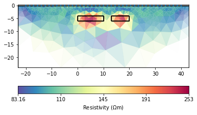
If I expand the overall size like change the 'world' and refine the mesh ‘area=0.1’
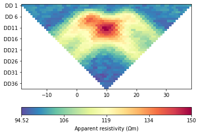
world = mt.createWorld(start=[-60, 0], end=[120, -30], worldMarker=True)
c1 = mt.createPolygon([[0, -4], [10, -4],[10, -6], [0, -6]],
isClosed=True, marker = 2, area=0.1)
c2 = mt.createPolygon([[13,-4], [20, -4], [20, -6], [13,-6]],
isClosed=True, marker = 3, area=0.1)
geom = c1+c2+world
pg.show(geom)
The result still have a large resistivity near the sensor
The last question, just like last issue#429. I only do 'mesh = mt.createGrid()' and input the vector 'vp' to each grid, without creating 'geom = createWorld/createPolygon' how to add sensors 'geom.createNode()'.
I will try mt.createParaMeshPLC(scheme)
, thanks for your help!
Can you try using an improved triangle quality of 34 or above?
import numpy as np
import pygimli as pg
import pygimli.meshtools as mt
import matplotlib.pyplot as plt
from pygimli.viewer import showMesh
from pygimli.physics import ert
world = mt.createWorld(start=[-60, 0], end=[120, -30], worldMarker=True)
c1 = mt.createPolygon([[0, -4], [10, -4],[10, -6], [0, -6]],
isClosed=True, marker = 2, area=5)
c2 = mt.createPolygon([[13,-4], [20, -4], [20, -6], [13,-6]],
isClosed=True, marker = 3, area=5)
geom = c1+c2+world
pg.show(geom)
mesh = mt.createMesh(geom,
area=5,
quality=34.3,
smooth=[2, 4]
)
showMesh(mesh, markers=True, showMesh=True);
scheme = ert.createData(elecs=np.linspace(start=-20, stop=40, num=41),
schemeName='dd')
for p in scheme.sensors():
geom.createNode(p)
geom.createNode(p - [0, 0.1])
rhomap = [[1, 100.],
[2, 500.],
[3, 500.]]
pg.show(mesh, data=rhomap, label=pg.unit('res'), showMesh=True)
ax, _ = pg.show(mesh, rhomap, colorBar=True, logScale=False, label='rh in Ωm')
pg.viewer.mpl.drawSensors(ax, scheme.sensors(), diam=1.0,
facecolor='white', edgecolor='black')
data = ert.simulate(mesh, scheme=scheme, res=rhomap, noiseLevel=0.01,
noiseAbs=1e-6, seed=1337)
pg.info(np.linalg.norm(data['err']), np.linalg.norm(data['rhoa']))
pg.info('Simulated data', data)
pg.info('The data contains:', data.dataMap().keys())
pg.info('Simulated rhoa (min/max)', min(data['rhoa']), max(data['rhoa']))
pg.info('Selected data noise %(min/max)', min(data['err'])*100, max(data['err'])*100)
data.remove(data['rhoa'] < 0)
pg.info('Filtered rhoa (min/max)', min(data['rhoa']), max(data['rhoa']))
data.save('tcfgz0simple.dat')
ert.show(data)
mgr = ert.ERTManager('tcfgz0simple.dat')
inv = mgr.invert(lam=50, verbose=True)
ax = mgr.showResult(colorBar=True,logScale=True)
pg.show(ax=ax, fillRegion=False, regionMarker=False)
The result of the modified code is shown in the figure above, thank you!
You need to add the electrodes to the geometry BEFORE you mesh it. Otherwise it will never be used. So you should shift the lines with for p in scheme.sensors():
(and the createData as well
) above the line mesh = mt.createMesh(geom
import numpy as np
import pygimli as pg
import pygimli.meshtools as mt
from pygimli.viewer import showMesh
from pygimli.physics import ert
world = mt.createWorld(start=[-60, 0], end=[120, -30], worldMarker=True)
c1 = mt.createPolygon([[0, -4], [10, -4], [10, -6], [0, -6]],
isClosed=True, marker=2, area=5)
c2 = mt.createPolygon([[13, -4], [20, -4], [20, -6], [13, -6]],
isClosed=True, marker=3, area=5)
scheme = ert.createData(elecs=np.linspace(start=-20, stop=40, num=41),
schemeName='dd')
geom = c1+c2+world
for p in scheme.sensors():
geom.createNode(p)
geom.createNode(p - [0, 0.1])
pg.show(geom)
mesh = mt.createMesh(geom,
area=5,
quality=34.3,
smooth=[2, 4]
)
showMesh(mesh, markers=True, showMesh=True)
rhomap = [[1, 100.],
[2, 500.],
[3, 500.]]
pg.show(mesh, data=rhomap, label=pg.unit('res'), showMesh=True)
ax, _ = pg.show(mesh, rhomap, colorBar=True, logScale=False, label='rh in Ωm')
pg.viewer.mpl.drawSensors(ax, scheme.sensors(), diam=1.0,
facecolor='white', edgecolor='black')
data = ert.simulate(mesh, scheme=scheme, res=rhomap, noiseLevel=0.01,
noiseAbs=1e-6, seed=1337)
pg.info(np.linalg.norm(data['err']), np.linalg.norm(data['rhoa']))
pg.info('Simulated data', data)
pg.info('The data contains:', data.dataMap().keys())
pg.info('Simulated rhoa (min/max)', min(data['rhoa']), max(data['rhoa']))
pg.info('Selected data noise %(min/max)', min(data['err'])*100,
max(data['err'])*100)
data.remove(data['rhoa'] < 0)
pg.info('Filtered rhoa (min/max)', min(data['rhoa']), max(data['rhoa']))
data.save('tcfgz0simple.dat')
ert.show(data)
mgr = ert.ERTManager('tcfgz0simple.dat')
inv = mgr.invert(lam=50, verbose=True)
ax, cb = mgr.showResult(colorBar=True, logScale=True)
pg.show(geom, ax=ax, fillRegion=False, regionMarker=False, fitView=False)
Wow thanks a lot! If I used established regular grid like createGrid
without createWorld like 'geom', I'm sorry for the aforementioned you may not have noticed.
‘’The last question, just like last issue#429. I only do 'mesh = mt.createGrid()' and input the vector 'vp' to each grid, without creating 'geom = createWorld/createPolygon' how to add sensors 'geom.createNode()'.’
I tried cross-hole ERT in a regular grid for example, so how to introduce the code
for electrode in scheme.sensors():
geom.createNode(electrode)
geom.createNode(electrode - [0, 0.1])
to encrypted monitoring points without 'geom'.
Example:
import numpy as np
import pygimli as pg
import pygimli.meshtools as mt
from pygimli.viewer import showMesh
from pygimli.physics import ert
import matplotlib.pyplot as plt
mesh = mt.createGrid(x=[0,1,2,3,4,5,6,7,8,9,10,11,12,13,14,15,16,17,18,19,20], y=[0,-1,-2,-3,-4,-5,-6,-7,-8,-9,-10,-11,-12,-13,-14,-15,-16,-17,-18,-19,-20])
_= pg.show(mesh, markers=True, showMesh=True)
print(mesh)
n = 21
borehole = np.ones((n, 2))*1
borehole_ = np.ones((n, 2))*19
borehole[:,1] = np.array([0,-1,-2,-3,-4,-5,-6,-7,-8,-9,-10,-11,-12,-13,-14,-15,-16,-17,-18,-19,-20]) # down to 23 m depth
borehole_[:,1] = np.array([0,-1,-2,-3,-4,-5,-6,-7,-8,-9,-10,-11,-12,-13,-14,-15,-16,-17,-18,-19,-20])
sensors = np.vstack([borehole,borehole_])
ax, _ = pg.show(mesh, markers=True, showMesh=True)
ax.plot(sensors[:,0], sensors[:,1], "mo")
rhomap=[100,100,100,100,100,100,100,100,100,300,300,100,100,100,100,100,100,100,100,100,100,100,100,100,100,100,100,100,100,310,310,100,100,100,100,100,100,100,100,100,100,100,100,100,100,100,100,100,100,320,320,100,100,100,100,100,100,100,100,100,100,100,100,100,100,100,100,100,100,330,330,100,100,100,100,100,100,100,100,100,100,100,100,100,100,100,100,100,100,330,330,100,100,100,100,100,100,100,100,100,100,100,100,100,100,100,100,320,340,340,340,340,320,100,100,100,100,100,100,100,100,100,100,100,100,100,100,320,500,500,500,500,320,310,100,100,100,100,100,100,100,100,100,100,100,100,320,100,100,500,500,100,320,100,100,100,100,100,100,100,100,100,100,100,100,100,320,100,100,100,100,100,320,100,100,100,100,100,100,100,100,100,100,100,100,300,310,100,100,100,100,100,310,100,100,100,100,100,100,100,100,100,100,100,100,100,310,100,100,300,310,310,310,310,310,300,100,100,100,100,100,100,100,100,100,100,310,100,100,310,500,500,500,500,500,310,100,100,100,100,100,100,100,100,100,100,310,100,100,300,100,500,500,500,100,310,100,100,100,100,100,100,100,100,100,100,100,300,100,300,100,100,500,100,100,300,100,100,100,100,100,100,100,100,100,100,100,100,100,300,100,100,100,100,100,300,100,100,100,100,100,100,100,100,100,100,100,300,100,300,100,100,100,100,100,100,100,100,100,100,100,100,100,100,100,100,100,100,100,300,100,100,100,100,100,100,100,100,100,100,100,100,100,100,100,100,100,100,300,100,100,100,100,100,100,100,100,100,100,100,100,100,100,100,100,100,100,100,100,100,100,100,100,100,100,100,100,100,100,100,100,100,100,100,100,100,100,100,100,100,100,100,100,100,100,100,100,100,100,100]
rhomap = np.asarray(rhomap)
pg.show(mesh, data=rhomap, label=pg.unit('res'), showMesh=True)
scheme = ert.createERTData(sensors,schemeName='dd')
print(scheme)
print(scheme.sensor(0))
np.column_stack((pg.x(scheme), pg.y(scheme)))
print(scheme["valid"])
data = ert.simulate(mesh, scheme=scheme, res=rhomap, noiseLevel=0.01,
noiseAbs=1e-6, seed=1337)
pg.info(np.linalg.norm(data['err']), np.linalg.norm(data['rhoa']))
pg.info('Simulated data', data)
pg.info('The data contains:', data.dataMap().keys())
pg.info('Simulated rhoa (min/max)', min(data['rhoa']), max(data['rhoa']))
pg.info('Selected data noise %(min/max)', min(data['err'])*100, max(data['err'])*100)
ert.show(data)
data.remove(data['rhoa'] < 0)
pg.info('Filtered rhoa (min/max)', min(data['rhoa']), max(data['rhoa']))
data.save('gcERT20.dat')
mgr = ert.ERTManager('gcERT20.dat')
inv = mgr.invert(data, mesh, secNodes=4, lam=10,verbose=True)
ax = mgr.showResult(colorBar=True,logScale=True)
pg.show(ax=ax, fillRegion=False, regionMarker=False)
Wow thanks a lot! If I used established regular grid like createGrid without createWorld like 'geom', I'm sorry for the aforementioned you may not have noticed.
I am sorry, but I can't get any meaning of this sentence. From
I only do 'mesh = mt.createGrid()' and input the vector 'vp' to each grid, without creating 'geom = createWorld/createPolygon' how to add sensors 'geom.createNode()'.’ I tried cross-hole ERT in a regular grid for example, so how to introduce the code
I am guessing that you want to include the electrode positions in a regular grid. As you specify the x and y vectors in mt.createGrid(x, y)
it is in your hands to define x and y accordingly. This works only if the positions are regular. If not I strongly recommend irregular triangle meshes.
Thanks a lot for your quick reply.
Yes, pyGIMLi can be used for crosshole ERT modelling and inversion. However I strongly recommend using a larger mesh further away from the electrodes (some of them are on the boundary, which leads to inaccuracies). There are two ways:
mesh=pg.createGrid
directly. Make sure electrodes are nodes. No geom
used.geom
with possible structures, add electrodes as nodes, and mesh it into a irregular triangle mesh by mesh=mt.createMesh(geom)
.The function ert.createData
is designed for linear electrode arrays such as surface profiles or a single borehole. For cross-borehole, there is a number of different arrays with good resolution properties. By applying a standard array to two boreholes you will have quadrupoles with zero or near-zero voltage gains, i.e. extremely large geometric factors. These are responsible for the strange effects. You should get rid of those by using data.remove(pg.abs(data["k"]) > kmax)
.
Ok, thank you very much, when I output the forward modeling data or consider the forward modeling results, I can see that the monitoring scheme always simulates one side of the borehole first, and then switches to the second borehole, so I want to confirm is the following data correct? for example:
I believe that each sensor should be taken at the same height for the left and right boreholes, and then two sensors at intervals on one side should be selected for simulation. such as:
There is no such thing as a "correct" array. The first one is a dipole-dipole array that is not suitable for crosshole as there are a lot of small voltage gains. In crosshole there are many ideas for arrays that have a good tradeoff between signal-to-noise and resolution. Please have a look at the literature, e.g. El Hagrey (2012):
El Hagrey (2012): 2D Optimized Electrode Arrays for Borehole Resistivity Tomography and CO2 Sequestration Modelling, Pure Appl. Geophys. 169 (2012), 1283–1292, doi:10.1007/s00024-011-0369-0
Alright, thank you very much!
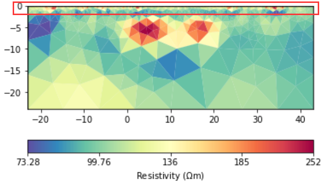
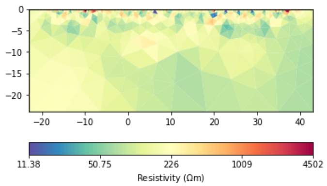
The forward and inversion results will have a large resistivity near the sensor. The larger the scale, the greater the resistivity. How to avoid abnormal values?
Other case: Looking forward to your reply! Thank you!