Latent experiment

[mtsokol]

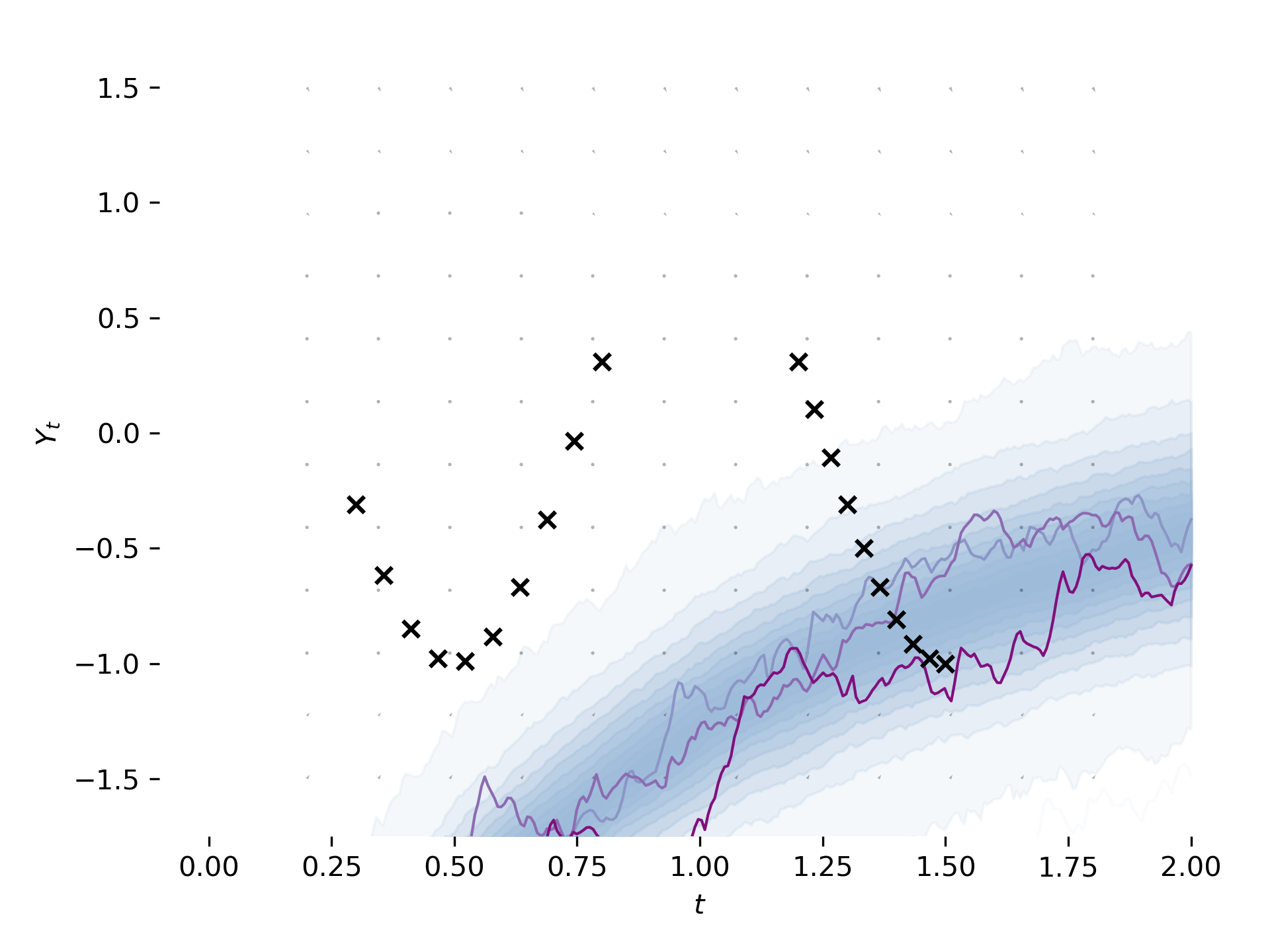
Hi!

Following next instructions in https://github.com/google-research/torchsde/pull/38#issuecomment-686559686 here's my idea for that - I've looked what flow exactly is for previous version available on master and hopefully recreated it.

That's a result after 300 iterations (still not similar to 300 in previous version):

WDYT?

btw. running it locally was still slow and burning laptop so I ended up running it on CGP instance (e2-highcpu-8) as I found they have student packs and got one iteration at 4sec.

[lxuechen]

I think now we're seeing something on the right track. The main issue here is that you should just take zs[-1, :, 1] as logqp to make it consistent with what we had before, as opposed to summing over the first dimension, which would mean inflating the KL divergence.

[mtsokol]

@lxuechen I've applied all comments and run it but it doesn't seem good after 400 iterations:

Regarding taking last entry of logqp - I've tracked existing implementation and in https://github.com/google-research/torchsde/blob/master/torchsde/_core/base_solver.py#L227 logqp is appended after each step and I don't see where only last entry is retrieved.

[lxuechen]

Regarding taking last entry of logqp - I've tracked existing implementation and in https://github.com/google-research/torchsde/blob/master/torchsde/_core/base_solver.py#L227 logqp is appended after each step and I don't see where only last entry is retrieved.

The version on master records the logqp penalty accumulated on each subinterval and returns a tensor of size (T-1, batch_size), where the first dimension indexes the subinterval. The design there was so that users may explicitly weight the penalty according to chronological order if they wanted to. So if we want the vanilla logqp (equal weighting among different subintervals), we would sum over the first dimension. You can see that the logqp term for each subinterval is reset to 0 at the beginning.

The current version with augmentation tracks the absolute quantity, so we only need to take the end result in order to get a value consistent with what we previously had.

[lxuechen]

Thanks for patiently addressing the issues I mentioned! I think this PR is just a few small fixes away from getting merged.

[mtsokol]

@lxuechen All done! Last question that I forgot to ask: Why in this example do we encode NN input as (sin(t), cos(t), y) instead of just (t, y)? As also with such formula second input is determined by the first one which seems redundant.

[lxuechen]

@lxuechen All done! Last question that I forgot to ask: Why in this example do we encode NN input as (sin(t), cos(t), y) instead of just (t, y)? As also with such formula second input is determined by the first one which seems redundant.

This is to mimic positional encoding in transformers. Also it's incorrect to say that the value of sine determines the value of cosine, e.g. sin(pi/4) == sin(3pi/4), but cos(pi/4) != cos(3pi/4). This is elementary trigonometric.

[mtsokol]

All done!

@lxuechen All done! Last question that I forgot to ask: Why in this example do we encode NN input as (sin(t), cos(t), y) instead of just (t, y)? As also with such formula second input is determined by the first one which seems redundant.

This is to mimic positional encoding in transformers. Also it's incorrect to say that the value of sine determines the value of cosine, e.g. sin(pi/4) == sin(3pi/4), but cos(pi/4) != cos(3pi/4). This is elementary trigonometric.

I was thinking about something completely different while writing this, not even looking at what functions are used, let's say because of current late night hour (embarrassment)

[lxuechen]

All done!

@lxuechen All done! Last question that I forgot to ask: Why in this example do we encode NN input as (sin(t), cos(t), y) instead of just (t, y)? As also with such formula second input is determined by the first one which seems redundant.

This is to mimic positional encoding in transformers. Also it's incorrect to say that the value of sine determines the value of cosine, e.g. sin(pi/4) == sin(3pi/4), but cos(pi/4) != cos(3pi/4). This is elementary trigonometric.

I was thinking about something completely different while writing this, not even looking at what functions are used, let's say because of current late night hour (embarrassment)

No worries! I understand that might happen at times.

[mtsokol]

Thanks for all the assistance once again! This or the following week I will try to do next small thing from milestone list (also started simple benchmark which I was asking earlier, will see how it goes).

(I thought about turning open source contributions into some simple master thesis to be able to spend more time on this but unfortunately I haven't found anyone interested in supervising it at uni for coming year).

---

Also I've got a question related to constraints of gradient computation (please let me know if it's inappropriate to ask here!) Some time ago I was learning about Physics Informed Neural Networks idea for solving PDEs from it's original paper and Tensorflow source code. I experimented with a small tweak - instead of learning whole solution u(x,t) with NN, I thought about introducing bspline base functions for solution like in FEM and using NN to learn it's coefficients. I've created full prototype: https://github.com/pierremtb/PINNs-TF2.0/pull/3 But eventually it just pull all coefficients close to zero and doesn't recreate desired shape.

As there's a heat equation example and PINNs use gradient descent it eventually computes higher order derivatives of Tensorflow's control flows like loops and ifs (used for choosing correct bsplines). (I also tried learning coefficients straight from GD but also failed)

So do you think that computing gradient of such complex logic might be unfeasible to acquire solution or there's no reason to say that and it's rather implemented incorrectly?

[lxuechen]

Sorry for the late response, as I've been incredibly busy lately.

Obviously, I'm not an expert on the specific models you described. What I may potentially comment on in an educated manner is the part about differentiating through control flow and obtaining high-order derivatives.

Since both TF eager-mode and Pytorch use tape-based systems, taking gradients through control flow shouldn't be a problem, even if that control flow is pure Python code (Python if-else, for, while statements). Obviously, things get tricky when you start with TF graph-mode and jitting/scripting PyTorch code, and things typically break without there being potential simple fixes. Obviously, this is only coming from my limited experience.

Second-order gradients typically aren't a problem either, if the specific computation can be grouped into Hessian-vector products, which can then be computed using just vector-Jacobian products. I haven't seen examples of taking gradients beyond the second-order in the ML literature so far.