 learning-chip
commented
2 years ago
learning-chip
commented
2 years ago A slightly cleaned-up script:
using Gridap
using CairoMakie

"""Extract node coordinates as 1D arrays from 2D regular mesh"""
function get_node_coords_2d(model)
    node_coords = model.grid.node_coords
    node_x = map(coords -> coords[1], node_coords)
    node_y = map(coords -> coords[2], node_coords)
    x_1d = node_x[1:end-1, 1]  # remove boundary node
    y_1d = node_y[1, 1:end-1]
    return x_1d, y_1d
end

"""Extract vector components from 2D nedelec field"""
function get_nedelec_comp_2d(uh)
    u_comps = [map(v -> v[i], uh.cell_dof_values) for i=1:4];
    u_comps_2d = map(u -> reshape(u, (n_1d, n_1d)), u_comps);
    ux = u_comps_2d[1]
    uy = u_comps_2d[3]
    return ux, uy
end

"""Plot separately two components of 2D nedelec field"""
function plot_nedelec_comp_2d(uh)
    model = uh.cell_field.trian.model
    x_1d, y_1d = get_node_coords_2d(model)
    ux, uy = get_nedelec_comp_2d(uh)

    fig = Figure(resolution=(600, 300))
    heatmap(fig[1, 1], x_1d, y_1d, ux)
    heatmap(fig[1, 2], x_1d, y_1d, uy)
    # TODO: add colorbar
    return fig
end

"""Plot arrows for 2D nedelec field """
function plot_nedelec_vector(uh; lengthscale=0.05)
    model = uh.cell_field.trian.model
    x_1d, y_1d = get_node_coords_2d(model)
    ux, uy = get_nedelec_comp_2d(uh)
    strength = sqrt.(ux.^2 + uy.^2)
    strength_1d = vec(strength)
    arrows(
        x_1d, y_1d, ux, uy,
        lengthscale=lengthscale,
        arrowcolor=strength_1d,
        linecolor=strength_1d
    )
end

"""Convert plain array of free values to visualizable field object"""
function free_to_field(x_free, V)
    xh = interpolate(x -> VectorValue(0, 0), V)
    xh.free_values[:] = x_free
    return xh
end
Example usage:
n_1d = 16
domain = (0, 1, 0, 1)
partition = (n_1d, n_1d)
model = CartesianDiscreteModel(domain, partition)
reffe = ReferenceFE(nedelec, 0)
V = FESpace(model, reffe)
uh = interpolate(x -> VectorValue(x[1] + x[2], x[2] - x[1]), V)

plot_nedelec_comp_2d(uh)  # plot separate components
plot_nedelec_vector(uh)  # plot vector field
# plot plain array of free values
x = rand(length(uh.free_values)) # some array, possibly from external solver
xh = free_to_field(x, V)
plot_nedelec_vector(xh) # works exactly the same as for `uh` aboveStill hacky with unnecessary duplicated calculations, but at least usable😅
 fverdugo
In order to visualize some Maxwell simulation results (without writing to VTK), I hacked some code to plot vector field with zeroth-order Nedelec element on quadrilateral mesh. Would it be useful to add to GridapMakie.jl?
Currently, plotting a field with Nedelec element seems unsupported:
simplexifycall,plot() returns empty figure. Probably because the plotting logic assumes unstructured mesh instead of Cartesian mesh?simplexifycall, the later lineV = FESpace(model, reffe)leads toThis function is not yet implemented. Not sure if related to gridap/Gridap.jl#413Error message:
Manually plot vector field with Nedelec element
This looks hacky and only works for zeroth-order Nedelec element + quadrilateral mesh. 2D and 3D are both okay. For high-order elements and other meshes, need a more generic way to find the location of each DoF and the orientation of each edge.
The resulting plot: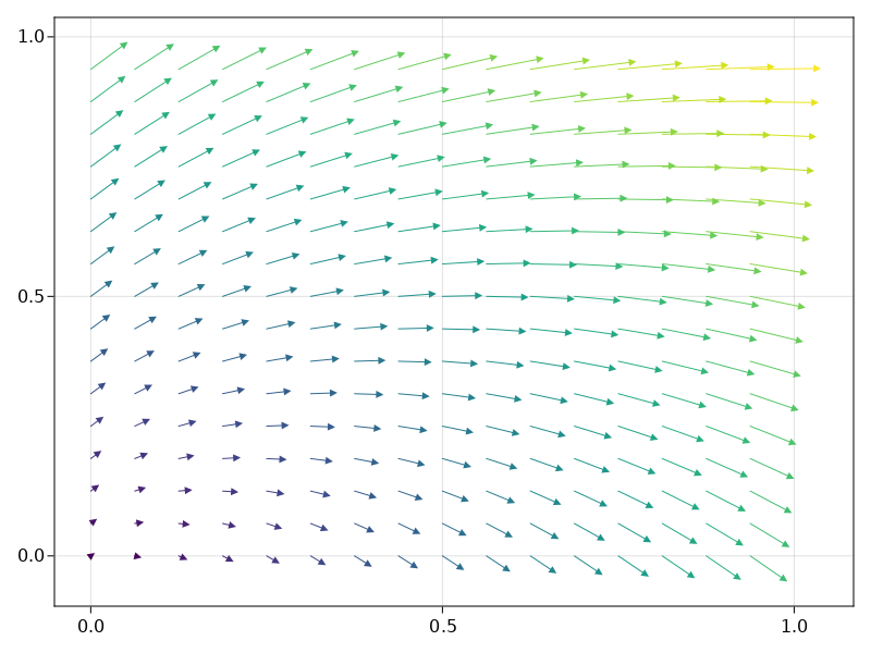
Makie
arrows()also works for 3D case.An additional hack, useful when using external linear solver to get approximate solution
x, and to visualize such solution (useful for checking the results of an approximate/iterative solver).A better way would be straightly figure out the location and orientation of each edge corresponding to free values, without querying
uh.cell_dof_values. But I haven't figured out how to do that...I'd like to clean up and improve those hacks, and hopefully contribute a more generic solution for vector plotting. Suggestions are welcome :)