walker_glm(distribution = "binomial") forecasts a large excess of 0.5

[wpetry]

brief description of the model

I'm attempting to implement a pure random walk model in which the underlying data generating process is described by where y is a proportion between [0, 1]. The underlying state, y, is observed through counts of successes and failures using a logit link.

description of the unexpected behavior

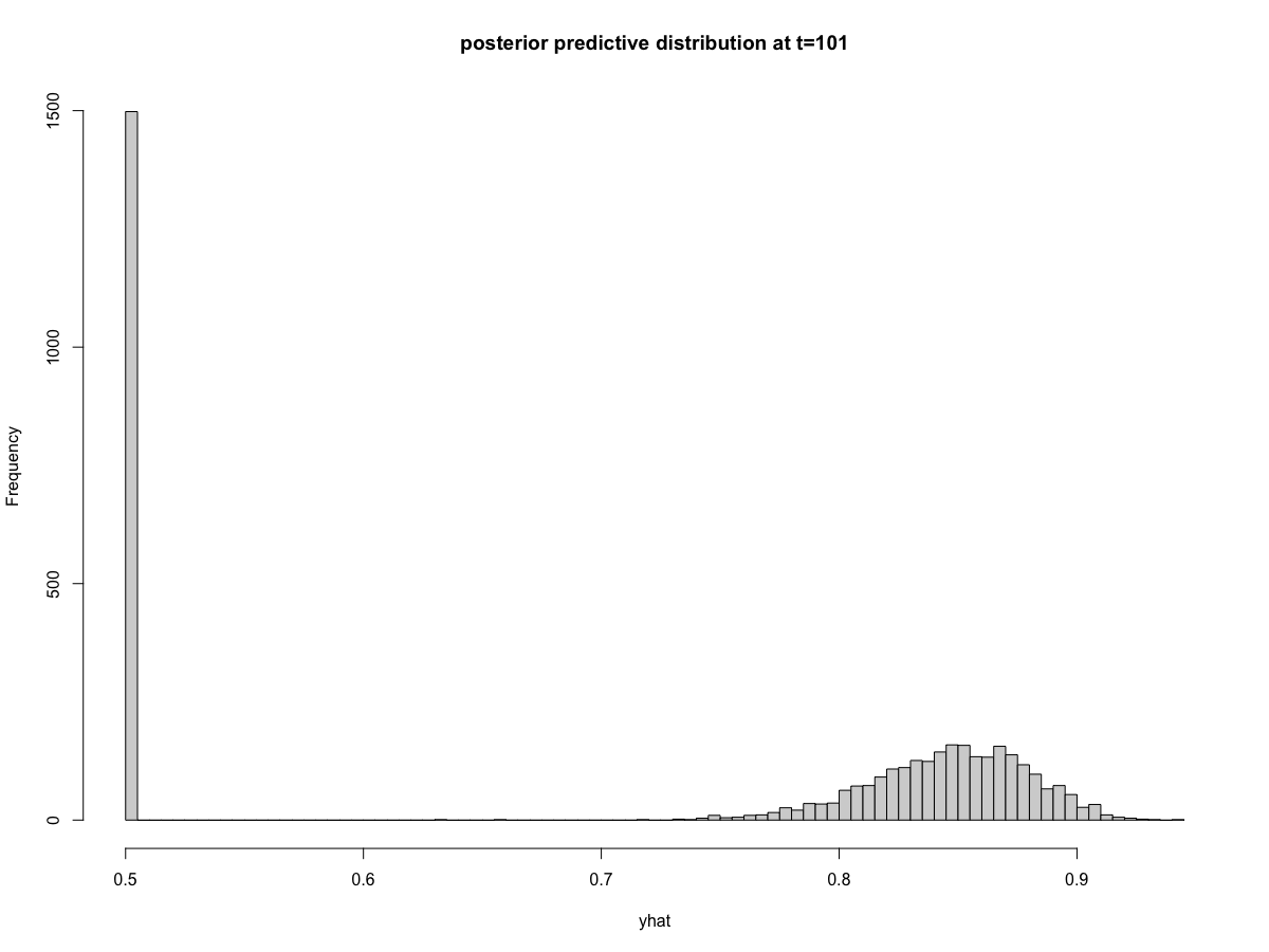
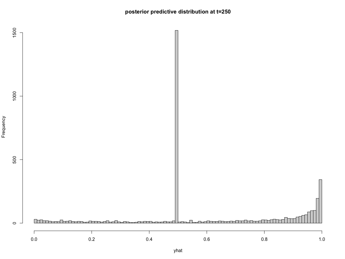
The problem is that when I forecast from model fit with walker_glm(distribution = "binomial"), the prediction intervals behave strangely. Specifically, there is a very large excess of predictions at exactly 0.5 (corresponding to zero on the logit scale). The remainder of the posterior predictive distribution aligns with my expectations. We can visualize this problem in the posterior predictive intervals,

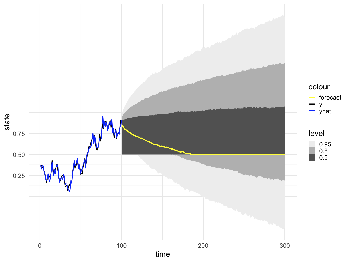
and in the posterior predictions at time=101

and time=250

potentially important clue

I noticed that all timepoints appear to have the same exact number of posterior predictions that equal 0.5 (again, this is the same as saying zero on the logit scale). You can see this in the histograms above where 1498 draws equal 0.5 at both t=101 and t=250 (the exact count will vary depending on the random seed). The reprex below provides code that shows this is true across all time points. I can't think of a mechanism that would cause consistency of posterior draws across every time point.

reprex

We can simulate nt=100 time steps of the true data y, the number of observed successes succ out of nobs trials, and the estimated state on the probability scale yhat as:

# preliminaries
library(walker)
library(tidyverse)
library(ggedit)  # used later to remove count layer from plot_predict()

## simulate data generating process
## (a random walk proportion, estimated from observed successes)
# parameters
sigma <- 0.25  # standard deviation of the 'step size' on logit scale

# sample sizes
nt <- 100  # duration of observed timeseries
nobs <- 300  # total number of observations of events with probability 'y'

# generate latent process data
set.seed(32101)
rw <- cumsum(rnorm(nt, 0, sigma))  # random walk process on logit scale
y <- plogis(rw)  # timeseries of _true_ Pr(success)

# simulate observations of latent process
succ <- rbinom(nt, nobs, y)  # timeseries of observed successes
yhat <- succ / nobs  # timeseries of _estimated_ Pr(success)

plot.ts(y, ylim = c(0, 1))  # true Pr(success)
lines(yhat, col = "blue")  # estimated Pr(success)

dat <- data.frame(time = 1:nt, rw, y, succ, nobs, yhat)

We can then fit the model using walker_glm() with a very weak prior on the value of yhat at time=0, and confirm that the parameters are correctly recovered:

## pick a flat prior for the observed proportions
plot(density(plogis(rnorm(1e6, mean = 0, sd = 1.45))))

## fit a pure random walk model to the data (takes ~90s)
rwfit <- walker_glm(succ ~ 0 +  # don't fit an overall intercept
                      rw1(~ 0,  # don't fit a time-varying intercept or covariates
                          beta = c(0, 1.45),  # prior: Normal(0,1.45) on observation at t0 (logit scale)
                          sigma = c(0, 2)),  # prior: Half-Normal(0,2) on 'sigma'
                    u = dat$nobs,  # total number of plants counted
                    distribution = "binomial",  # model ratio from count data
                    data = dat, iter = 2000, warmup = 1000, chains = 4, cores = 4)

## check convergence
rwfit
pp_check(rwfit)

## check that sigma is correctly recovered
sigma_est <- unlist(lapply(rwfit[["stanfit"]]@sim[["samples"]], function(x) x[["sigma_rw1[1]"]]))
hist(sigma_est)
abline(v = sigma, col = "blue")

Finally, make the forecast for times 101 to 300:

## forecast the model from times 101:300
ndat <- data.frame(time = 1:length(101:300))

rwfc <- predict(rwfit, newdata = ndat, u = nobs)

## plot forecast using internal walker function
plot_predict(rwfc) %>%
  remove_geom("line", 2)

## re-plot with tidybayes to show multiple posterior intervals
plotdat <- as.data.frame(rwfc[["y_new"]]) %>%
  rownames_to_column(var = "time") %>%
  pivot_longer(-time, names_to = ".iter", values_to = "yhat") %>%
  mutate_if(is.character, as.integer)

ggplot(plotdat, aes(x = time, y = yhat))+
  stat_lineribbon(aes(color = "forecast"))+
  geom_line(data = dat, aes(y = y, color = "y"), size = 1)+
  geom_line(data = dat, aes(y = yhat, color = "yhat"), size = 1)+
  scale_y_continuous(name = "state", trans = scales::logit_trans())+
  scale_color_manual(values = c("yellow", "black", "blue"))+
  scale_fill_brewer(palette = "Greys")+
  theme_minimal(base_size = 20)

## look at forecast posterior at t=101
plotdat %>%
  filter(time == 101) %>%
  pull(yhat) %>%
  hist(100, main = "posterior predictive distribution at t=101",
       xlab = "yhat")

## look at forecast posterior at t=250
plotdat %>%
  filter(time == 250) %>%
  pull(yhat) %>%
  hist(100, main = "posterior predictive distribution at t=250",
       xlab = "yhat")

# count the number of yhat == 0.5 at each time point
plotdat %>%
  mutate(test = yhat==0.5) %>%
  group_by(.$time) %>%
  summarize(count = sum(test))

Thank you, @helske, for your work on this package to make state space modeling intuitive and efficient.

[wpetry]

I repeated the model after changing the rw1 formula from ~0 to ~1. I worried that fitting a zero intercept here may have forced the predictions to instead of using the current state as in . The unexpected behavior (excess 0.5) persists despite this change.

[helske]

Thanks for a good example. I will get back to this tomorrow, there seems to be an issue with the underlying C++ function as using predict(rwfit, newdata = ndat, u = nobs,type="response") gives an out-of-bounds error.

And there seems to be an issue with the plot_predict as well regarding whether to plot observations or means which needs some attentions.

[wpetry]

Thanks for looking into this. I'm still a little confused about the correct way to specify the RHS of the rw1 formula for this data generating process. Would you please share the correct model code once the issue is resolved?

You're right about the opportunity to add a feature to plot_predict when working with non-Gaussian errors. I'll open a separate issue since this is unrelated to the bug described here.

[helske]

Ok, there was a very simple indexing bug with the predict function which for some weird reason I hadn't spotted before, so I managed to fix this already.

[wpetry]

Wow, thanks for turning this around so quickly. I'm glad it was a relatively easy fix. Everything is now behaving as expected on my end.