jl749 commented 2 years ago

Deep learning is EXPENSIVE

e.g. train ResNet50 with ImageNet dataset for 80 epochs 80 1.3M images 7.7B ops per img

Solution?

Data Parallelism (large batch training)
Communication optimization
Model Parallelism

Large batch training

process more samples (imgs) per iteration (scale training of deep neural networks to larger numbers of accelerators and reduce the training time)

but what are the costs?

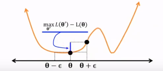
before we talk about it. let's look into Flatness, Generalization and SGD (https://www.inference.vc/sharp-vs-flat-minima-are-still-a-mystery-to-me/) the loss surface of deep nets tends have many local minima. (different generalization performance) "Interestingly, stochastic gradient descent (SGD) with small batchsizes appears to locate minima with better generalization properties than large-batch SGD." (https://medium.com/geekculture/why-small-batch-sizes-lead-to-greater-generalization-in-deep-learning-a00a32251a4f)

how do we predict generalization properties? Hochreiter and Schmidhuber (1997): suggested that the flatness of the minimum is a good measure (e.g. think why we use cosine annealing)

Sharp Minima Can Generalize For Deep Nets (counter relation between generalization and flatness)

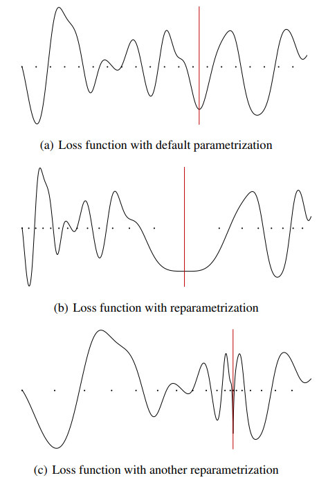
https://arxiv.org/pdf/1703.04933.pdf https://vimeo.com/237275513 However, flatness is sensitive to reparametrization (Dinh et al (2017)): we can reparametrize a neural network without changing its outputs (observational equivalence) while making sharp minima look arbitrarily flat and vice versa. --> flatness alone cannot explain or predict good generalization

non-negative homogeneity (neyshabur 2015)

e.g. ReLU

observational equivalence

different parameters but same output e.g. input @ A @ B == input @ -A @ -B e.g. alpha-scale transform

measure flatness

epsilon-flatness (Hochreiter and Schmidhuber (1997)) blue line represent Θ's flatness
epsilon-sharpness (Keskar et al. (2017))

On Large-Batch Training for Deep Learning: Generalization Gap and Sharp Minima (Keskar et al. (2017))

https://arxiv.org/pdf/1609.04836.pdf https://medium.com/geekculture/why-small-batch-sizes-lead-to-greater-generalization-in-deep-learning-a00a32251a4f large-batch methods tend to converge to sharp minimizers. In contrast, small-batch methods consistently converge to flat minimizers (this is due to the inherent noise in the gradient estimation)

sharp minima causes generalization gap between training and testing.

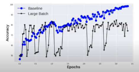
e.g. LSTM on MNIST dataset (baseline_batch: 256, large_batch: 8192)

[X] enumerate evidences

cross entropy loss against the sharpness (network F & network C) as our learners mature (loss reduces) the sharpness on the Large Batch learners increases

“For larger values of the loss function, i.e., near the initial point, SB and LB method yield similar values of sharpness. As the loss function reduces, the sharpness of the iterates corresponding to the LB method rapidly increases, whereas for the SB method the sharpness stays relatively constant initially and then reduces, suggesting an exploration phase followed by convergence to a flat minimizer.”

"Look at how quickly the networks converge to their testing accuracies"

if training-testing gap was due to a overfitting, we would not see the consistently lower performance of the LB methods. Instead by stopping earlier, we would avoid overfitting, and the performances(LB_testing <--> SB_testing) would be closer. (this is not what we observed) ==> "generalization gap is not due to over-fitting"

smaller batches are generally known to regularize, noise in the sample gradients pushes the iterates out of the basin of attraction of sharp minimizers the noise in large-batch is not sufficient to cause ejection from the initial basin leading to convergence to a sharper minimizer

jl749 commented 2 years ago

LAMB

https://krishansubudhi.github.io/deeplearning/2019/09/21/LambPaperDisected.html https://www.youtube.com/watch?v=dAumeKmPhDE https://www.youtube.com/watch?v=kwEBP-Wbtdc

Difficulties of Large-Batch Training

when λ is large, the update ||λ ∗ ∇L(wt)|| can become larger than ||wt||, and this can cause the training process to diverge. --> this is particularly problematic with larger mini-batch sizes which require higher learning rates to compensate for fewer training updates!! (large batch size ==> less frequent updates ==> reduced epochs)

Weight-Gradient ratios (||w|| / ||g||) can be a good indication

Layer1 has small ||w|| and large ||g||

if we use unified lr, λ = 100 Layer6: W = 6.4 - 100 0.005 (OK) Layer1: W = 0.098 - 100 0.017 (Diverge)

==> solution: assign unique learning rate for each layer

how is trust ratio defined?

weight_norm / gradient_norm + decay

benefits:

Weight-Gradient ratios provides robustness to exploding/banishing gradients (1 / ||g||)
Normalization of this form (||w|| // ||g||) essentially ignores the size of the gradient (adding a bit of bias) and is particularly useful in large batch settings where the direction of the gradient is largely preserved. (enables large learning rate)

y-asix = iteration x-axis = trust ratio z-axis = frequency

[ ] TODO: Lipschitz constants

jl749 commented 2 years ago

Accurate, Large Minibatch SGD: Training ImageNet in 1 Hour (https://arxiv.org/abs/1706.02677)

fixed num of epoechs --> fixed flops (see 2.1 for the interpretation)

warmup

for j, x in enumerate(optimizer.param_groups):
    # bias lr falls from 0.1 to lr0, all other lrs rise from 0.0 to lr0
    # lf = lambda x: (1 - x / epochs) * (1.0 - hyp['lrf']) + hyp['lrf']  # linear
    x['lr'] = np.interp(ni, xi, [hyp['warmup_bias_lr'] if j == 0 else 0.0, x['initial_lr'] * lf(epoch)])
    if 'momentum' in x:
        x['momentum'] = np.interp(ni, xi, [hyp['warmup_momentum'], hyp['momentum']])

lr0: 0.01 # initial learning rate

during the warmup for-loop

bias lr: 0.1 (warmup_bias_lr) --> 0.01 (initial lr) weight lr: 0 --> 0.01

https://stackoverflow.com/questions/55933867/what-does-learning-rate-warm-up-mean

https://arxiv.org/abs/1812.01187

==> Learning rate warm-up strategy empirical study shows that learning rate scaling heuristics with the batch size do not hold across all problems or across all batch sizes

jl749 commented 2 years ago

One weird trick for parallelizing convolutional neural networks (https://arxiv.org/pdf/1404.5997.pdf)

model parallelism

In model parallelism, whenever the model part (subset of neuron activities) trained by one worker requires output from a model part trained by another worker, the two workers must synchronize

efficient when the amount of computation per neuron activity is high (because the neuron activity is the unit being communicated) e.g. Linear layers contain about 5~10% of the computations, about 95% of the parameters, and have small representations

data parallelism

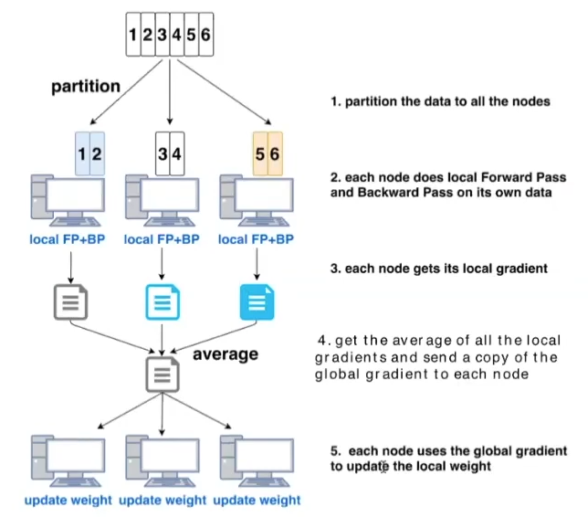
splitting a batch of data across multiple devices and then aggregating and applying the resulting gradients. (requires fast communication between devices, but also requires that large batches are alogrithmically effective)

In data parallelism the workers must synchronize model parameters (or parameter gradients) to ensure that they are training a consistent model.

efficient when the amount of computation per weight is high (because the weight is the unit being communicated) e.g. Conv layers cumulatively contain about 90~95% of the computation, about 5% of the parameters, and have large representations

how is batch size related?

we can make data parallelism arbitrarily efficient if we are willing to increase the batch size (because the weight synchronization step is performed once per batch)

[ ] TODO: read more about data/model parallelism

jl749 commented 2 years ago

An Empirical Model of Large-Batch Training

https://www.youtube.com/watch?v=wziA2TabG_8 https://openai.com/blog/science-of-ai/ https://www.reddit.com/r/MachineLearning/comments/8e9x8g/r_180407612_revisiting_small_batch_training_for/

batch_size: domain dependent (experience based...) e.g. RL can use millions BS while img recognition can use thousands

increasing BS == data parallelism computation efficiency vs time efficiency trade off (expensive and fast?, slow and efficient?) * training should parallelize almost linearly up to a batch size equal to the noise scale, after which there should be a smooth but relatively rapid switch to a regime where further parallelism provides minimal benefits

problem with model parallelism in general: main overhead becomes communication cost

When the batch size is very small, the approximation will have very high variance, and the resulting gradient update will be mostly noise. Applying a bunch of these SGD updates successively will average out the variance and push us overall in the right direction, but the individual updates to the parameters won’t be very helpful, and we could have done almost as well by aggregating these updates in parallel and applying them all at once (in other words, by using a larger batch size)

Minibatch gradient gives a noisy estimate of the true gradient, and larger batches give higher quality estimates

These results show that at fixed values of the loss, the noise scale does not depend significantly on model size.

When training neural networks, we typically process only a small batch of data at a time, which gives a noisy estimate of the true network gradient. We find that the gradient noise scale and we can approximately predict the maximum useful batch size heuristically When the noise scale is small, looking at a lot of data in parallel quickly becomes redundant, whereas when it is large, we can still learn a lot from huge batches of data. The noise scale typically increases by an order of magnitude or more over the course of training. Intuitively, this means the network learns the more “obvious” features of the task early in training and learns more intricate features later.

More difficult tasks and more powerful models on the same task will allow for more radical data-parallelism More powerful models have a higher gradient noise scale, but only because they achieve a lower loss. Thus, there’s some evidence that the increasing noise scale over training isn’t just an artifact of convergence, but occurs because the model gets better. If this is true, then we expect future, more powerful models to have higher noise scale and therefore be more parallelizable.

Faster training makes more powerful models possible and accelerates research through faster iteration times.

[ ] TODO: equation reading + code reading https://colab.research.google.com/drive/1C83B2crZ5QSYhIYhZ7CJMJ4al6Q8nP4U#scrollTo=QF7jQEvhfGvs https://github.com/dhuynh95/fastai_bs_finder/blob/master/bs_finder.ipynb

jl749 commented 2 years ago

Adam

https://towardsdatascience.com/adabelief-optimizer-fast-as-adam-generalizes-as-good-as-sgd-71a919597af If the gradients are all pointing in different directions (high variance), we’ll take a small, cautious step. Conversely, if all the gradients are telling us to move in the same direction, the variance will be small, so we’ll take a bigger step in that direction.

weight decay

https://towardsdatascience.com/this-thing-called-weight-decay-a7cd4bcfccab

jl749 commented 2 years ago

Weight Initialization

throughout the neural network

the mean of the activations should be zero
the variance of the activations should stay the same across

think about batchnrom layer in deep neural network

it resolves the scaling problem (e.g RetinaNet splits heads for different predictions, it wouldn't make sense to predict bbox and class in the same head (different number range))

The motivating intuition for this is in two parts; for the forward pass, ensuring that the variance of the activations is approximately the same across all the layers of the network allows for information from each training instance to pass through the network smoothly. Similarly, considering the backward pass, relatively similar variances of the gradients allows information to flow smoothly backwards. This ensures that the error data reaches all the layers, so that they can compensate effectively, which is the whole point of training. https://mnsgrg.com/2017/12/21/xavier-initialization/

Xavier Initialization

Justification for Xavier initialization

https://www.askpython.com/python/normal-distribution

jl749 commented 2 years ago

Property of an objective function (Lipschitz continuous gradient)

what's the property requirements for an objective functions? objective function: minimize or maximize under a constraint (R^n)

we have a differentiable function AND there is a constant L (positive) that defines correlation between distance from point A' gradient to point B's gradient and distance from point A to point B ===> function is Lipschitz continuous

Alt Text

so what is the intuition behind this?

https://www.youtube.com/watch?v=p-8FK2ldGZo

jl749 commented 2 years ago

https://leimao.github.io/blog/Data-Parallelism-vs-Model-Paralelism/

jl749 / LAMB_optimizer

Paper Reading #1

Deep learning is EXPENSIVE

Solution?

Large batch training

Sharp Minima Can Generalize For Deep Nets (counter relation between generalization and flatness)

non-negative homogeneity (neyshabur 2015)

observational equivalence

measure flatness

On Large-Batch Training for Deep Learning: Generalization Gap and Sharp Minima (Keskar et al. (2017))

LAMB

Difficulties of Large-Batch Training

how is trust ratio defined?

benefits:

Accurate, Large Minibatch SGD: Training ImageNet in 1 Hour (https://arxiv.org/abs/1706.02677)

warmup

during the warmup for-loop

One weird trick for parallelizing convolutional neural networks (https://arxiv.org/pdf/1404.5997.pdf)

model parallelism

data parallelism

how is batch size related?

An Empirical Model of Large-Batch Training

Adam

weight decay

Weight Initialization

Xavier Initialization

Property of an objective function (Lipschitz continuous gradient)

so what is the intuition behind this?