 lululxvi
commented
3 years ago
lululxvi
commented
3 years ago Normalize your PDE such that the boundary temperature is 0 and 1, not 100.
Closed SebasTouristTrophyF closed 3 years ago
lululxvi
commented
3 years ago Normalize your PDE such that the boundary temperature is 0 and 1, not 100.
 loubnabnl
commented
3 years ago
loubnabnl
commented
3 years ago @SebasTouristTrophyF I run your code and scaled the output of the neural network using the command line net.apply_output_transform(lambda x, y: y * 100)
and it works now!
k=9.7e-5 #thermal diffusivity
def pde(x, y):
    dy_x = tf.gradients(y, x)[0]
    dy_x, dy_t = dy_x[:, 0:1], dy_x[:, 1:2]
    dy_xx = tf.gradients(dy_x, x)[0][:, 0:1]
    return dy_xx - k*dy_t    # Heat conduction equation

geom = dde.geometry.Interval(0, 1)
timedomain = dde.geometry.TimeDomain(0, 5)
geomtime = dde.geometry.GeometryXTime(geom, timedomain)

def func(x):
    return -100 * x[:, 0:1] + 100

ic = dde.IC(geomtime, lambda x: np.full_like(x[:, 0:1], 0), lambda _, on_initial: on_initial)
bc = dde.DirichletBC(geomtime, func, lambda _, on_boundary: on_boundary)    # both sides -> dirichlet boundary condition -> fix value

data = dde.data.TimePDE(geomtime, pde, [bc, ic], num_domain=2500, num_boundary=500, num_initial=500, num_test=5000)
layer_size = [2] + [50] * 3 + [1]
activation = "tanh"
initializer = "Glorot uniform"
net = dde.maps.FNN(layer_size, activation, initializer)
net.apply_output_transform(lambda x, y: y * 100)
model = dde.Model(data, net)
model.compile("adam", lr=1.0e-3,loss_weights=[1, 1, 1])
model.train(epochs=50000)
model.compile("L-BFGS-B")
losshistory, train_state = model.train()
dde.saveplot(losshistory, train_state, issave=True, isplot=True)

if __name__ == "__main__":
    main()

 SebasTouristTrophyF
commented
3 years ago
SebasTouristTrophyF
commented
3 years ago Normalize your PDE such that the boundary temperature is 0 and 1, not 100.
Thanks for your pompt reply! I'm trying to solve the problem like this. Best regards
SebasTouristTrophyF
commented
3 years ago @SebasTouristTrophyF I run your code and scaled the output of the neural network using the command line
net.apply_output_transform(lambda x, y: y * 100)and it works now!k=9.7e-5 #thermal diffusivity def pde(x, y): dy_x = tf.gradients(y, x)[0] dy_x, dy_t = dy_x[:, 0:1], dy_x[:, 1:2] dy_xx = tf.gradients(dy_x, x)[0][:, 0:1] return dy_xx - k*dy_t # Heat conduction equation geom = dde.geometry.Interval(0, 1) timedomain = dde.geometry.TimeDomain(0, 5) geomtime = dde.geometry.GeometryXTime(geom, timedomain) def func(x): return -100 * x[:, 0:1] + 100 ic = dde.IC(geomtime, lambda x: np.full_like(x[:, 0:1], 0), lambda _, on_initial: on_initial) bc = dde.DirichletBC(geomtime, func, lambda _, on_boundary: on_boundary) # both sides -> dirichlet boundary condition -> fix value data = dde.data.TimePDE(geomtime, pde, [bc, ic], num_domain=2500, num_boundary=500, num_initial=500, num_test=5000) layer_size = [2] + [50] * 3 + [1] activation = "tanh" initializer = "Glorot uniform" net = dde.maps.FNN(layer_size, activation, initializer) net.apply_output_transform(lambda x, y: y * 100) model = dde.Model(data, net) model.compile("adam", lr=1.0e-3,loss_weights=[1, 1, 1]) model.train(epochs=50000) model.compile("L-BFGS-B") losshistory, train_state = model.train() dde.saveplot(losshistory, train_state, issave=True, isplot=True) if __name__ == "__main__": main()
Thanks, You're so nice! I'm reading your modified code to find out some helpful patterns for the future application. Thanks again for your selfless help! Best regards
SebasTouristTrophyF
commented
3 years ago @SebasTouristTrophyF I run your code and scaled the output of the neural network using the command line
net.apply_output_transform(lambda x, y: y * 100)and it works now!k=9.7e-5 #thermal diffusivity def pde(x, y): dy_x = tf.gradients(y, x)[0] dy_x, dy_t = dy_x[:, 0:1], dy_x[:, 1:2] dy_xx = tf.gradients(dy_x, x)[0][:, 0:1] return dy_xx - k*dy_t # Heat conduction equation geom = dde.geometry.Interval(0, 1) timedomain = dde.geometry.TimeDomain(0, 5) geomtime = dde.geometry.GeometryXTime(geom, timedomain) def func(x): return -100 * x[:, 0:1] + 100 ic = dde.IC(geomtime, lambda x: np.full_like(x[:, 0:1], 0), lambda _, on_initial: on_initial) bc = dde.DirichletBC(geomtime, func, lambda _, on_boundary: on_boundary) # both sides -> dirichlet boundary condition -> fix value data = dde.data.TimePDE(geomtime, pde, [bc, ic], num_domain=2500, num_boundary=500, num_initial=500, num_test=5000) layer_size = [2] + [50] * 3 + [1] activation = "tanh" initializer = "Glorot uniform" net = dde.maps.FNN(layer_size, activation, initializer) net.apply_output_transform(lambda x, y: y * 100) model = dde.Model(data, net) model.compile("adam", lr=1.0e-3,loss_weights=[1, 1, 1]) model.train(epochs=50000) model.compile("L-BFGS-B") losshistory, train_state = model.train() dde.saveplot(losshistory, train_state, issave=True, isplot=True) if __name__ == "__main__": main()
Hi @lululxvi @loubnabnl ,
Another set of questions for this old issue. Since I'm trying to get a transient solution for the 1-D heat conduction problem, but it seems that the modified code of Loubna has produced a solution of steady state (time-independent). That means, in the dimension of time all the temp distributions along x-direction are the same (except the initial condition).

So my set of questions are:
From my understanding, compared with HFM, what Dr. Lu Lu has done in DeepXDE goes a step further. In other words, DeepXDE is closer to the essence of this matter. That means, relying on the DeepXDE, we largely do not need a data set which on the one hand has the sample points with their coordinate while on the other hand also possesses the exact numerical calculated state values or measured ones as the labels (for computing the loss), all we need is only a set of sample points with their coordinate. This is because, different from the traditional supervised deep learning method, DeepXDE does not explicitly contain the labels. More specifically, the PINN method implicitly includes the labels (exact results) through the process of implementing the PDEs into neural network (giving the labels set in the form of PDE). The above is a very lengthy description, relying on it, I just want to express, in my understanding DeepXDE does not need to be given a reference solution/result. Therefore, I was a little surprised (not so surprised XD) when I saw that some examples still contain functions for reference solutions (??? not sure, e.g. the series of 1d-diffusion examples). So my first question is: do we need to give reference solutions in DeepXDE? If the answer is yes, what's the purpose? Accelerate the training? After that, we all know that many problems which require numerical computing actually have no analytical solutions. I also think that not having to give an analytical or numerical solution firstly is a huge advantage of PINN or DeepXDE.
Back to the question itself: the code listed before is modified based on the Burgers equation example. The BE example proves the many advantages of DeepXDE, e.g. it's a transient/time-dependent problem without giving a reference solution but the final result shows that the learning result of BE can be said to be perfect. Therefore, it is difficult for me to understand why the training results in this issue seem to be steady-state, in other words, time-independent. What's wrong with the code? Should I give a reference solution in the code, otherwise this problem will be difficult to be trained effectively?
Many thanks for your help Looking forward to your reply
lululxvi
commented
3 years ago SebasTouristTrophyF
commented
3 years ago
- Yes. DeepXDE is in some sense "unsurprised" and do not need label. You don't need to give the reference solution. The reference solutions in the examples are only used to check the accuracy of the solution obtained from DeepXDE.
- There is one problem in your setup. The IC is T=0, but the left BC is T=100, then what is T(x=0, t=0)? It is not well-defined. This may not be an issue in traditional numerical methods, but in PINNs it matters. Modify your IC or BC such that they are consistent, e.g., let the IC be T(x,t=0) = 100*(1-x)^2.
Thanks for the pompt reply :-). I've modified the IC and then get some logical results. However, it's based on a simplified pre set :p. Since I've found that this thermal issue and its corresponding PINN are very sensitive to the values' range (Just like what you've suggested before, it needs strict normalization. You can also note that in the following figure increasing of temperature happened within a very short time period). Therefore I decided to get the logical results firstly, and then keep tuning the code to get what I want.


SebasTouristTrophyF
commented
3 years ago A set of improved sim. results with the simplified pre set.
I use the old BC & IC, since I found that the x=0 point was not sampled by the IC. On the other side the x=0, t=1 point was sampled by the BC. Thus this IC & BC pair should lead to logical results:
 The simplified pre set makes the visualisation more obvious & beautiful:

 Letmesleepp
commented
2 years ago
Letmesleepp
commented
2 years ago @loubnabnl I'm sorry to bother you, but here's my question: How did you get the coefficientk=9.7e-5 #thermal diffusivity?
I'm now trying to rescale my code. If you can give me more details about rescaling problem, I'll very appreciate you.
loubnabnl
commented
2 years ago Hello @Letmesleepp , the value of k comes from physics, it's the thermal diffusivity of Aluminuim, you can find a table in the following link with the values of k for different materials: https://www.engineersedge.com/heat_transfer/thermal_diffusivity_table_13953.htm.
Hi Lu @lululxvi ,
First of all, thanks for providing such a powerful tool set so that we can adopt it to simulate various physical problems.
For above issue, I've almost gone through all the related issues in this reporitory. However, I can still not understand how to define right boundary conditions for the 1-D heat transfer problem (with both sides the temperature being fixed).
In my issue, I want to get the transient solution for such a case: for an 1-D problem with pure heat conduction, i.e. its corresponding pde should be:
In this case, we has a e.g. 1m tube with its left side possesses a fixed temperature of 100 °C, its right side has a fixed temperature of 0 °C. At the beginning, temperature of the rest part is also 0 °C. i.e. BCs should be: (Dirichlet) T(x=0) = e.g. 100 (Dirichlet) T(x=1) = e.g. 0 IC should be: T(t=0) = 0
Obviously, its logical solution should be like this: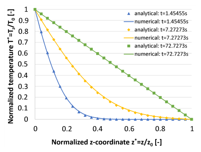
and this
However, with following codes my results are always: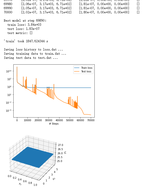
That means, although the listed training and test loss decreased simultaneously, the curve of training loss remain almost unchanged after about 10000 epochs. And the test part is also illogical.
from __future__ import absolute_importfrom __future__ import divisionfrom __future__ import print_functionimport numpy as npimport deepxde as ddefrom deepxde.backend import tfdef main():# constsheat_lamb = 3.2rho_m = 2500c_v = 1000I feel very confused and don't know where is wrong. Looking forward to your reply.