Problem solving 2d NS

[ethanshoemaker]

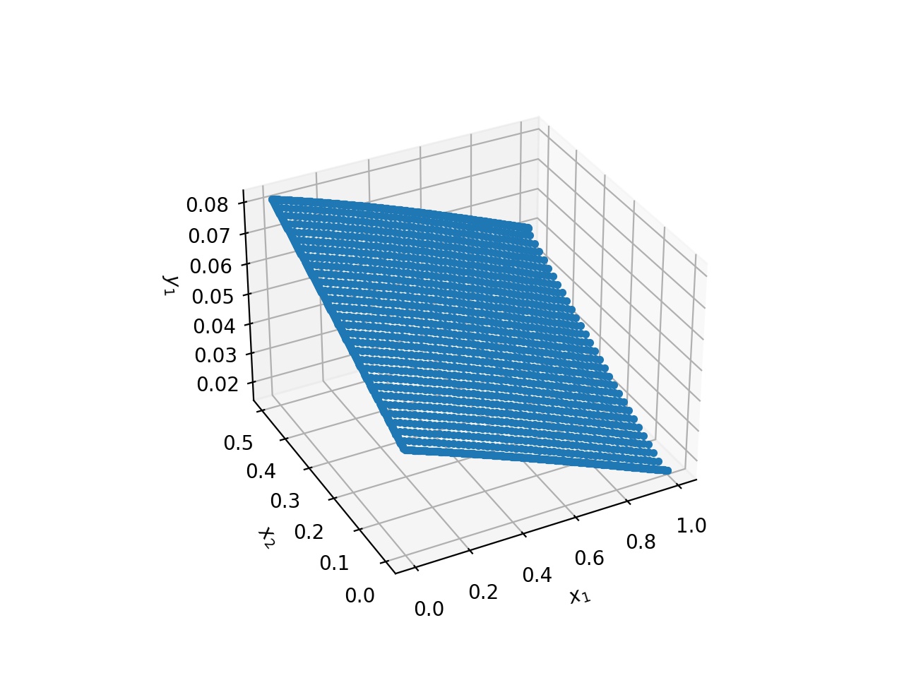
Hi Lu Lu, I am attempting a basic 2d flow (steady state, incompressible) problem through a pipe-like geometry. My losses are very low (lowest around 1e-7, highest around 1e-2), but the plots are no good. I would appreciate a second set of eyes. Here is my code. I've attached my plot of x-direction velocity as reference. I am also wondering how I can plot a colormap instead of traditional plot.

import deepxde as dde
from deepxde.backend import tf
import numpy as np
import matplotlib.pyplot as plt

geom = dde.geometry.geometry_2d.Rectangle([0,0],[1,0.5])
rho = 1000.
mu = 1e-3

def navier_stokes(x,y):
    u, v, p = y[:, 0:1], y[:, 1:2], y[:, 2:]
    u_x = dde.grad.jacobian(y, x, i=0, j=0)
    u_y = dde.grad.jacobian(y, x, i=0, j=1)
    v_x = dde.grad.jacobian(y, x, i=1, j=0)
    v_y = dde.grad.jacobian(y, x, i=1, j=1)
    p_x = dde.grad.jacobian(y, x, i=2, j=0)
    p_y = dde.grad.jacobian(y, x, i=2, j=1)
    u_xx = dde.grad.hessian(y, x, component=0, i=0, j=0)
    u_yy = dde.grad.hessian(y, x, component=0, i=1, j=1)
    v_xx = dde.grad.hessian(y, x, component=1, i=0, j=0)
    v_yy = dde.grad.hessian(y, x, component=1, i=1, j=1)
    continuity = u_x + v_y
    x_momentum = rho * (u * u_x + v * u_y) + p_x - mu * (u_xx + u_yy)
    y_momentum = rho * (u * v_x + v * v_y) + p_y - mu * (v_xx + v_yy)
    return [continuity, x_momentum, y_momentum]

def top_wall(x, on_boundary):
    return on_boundary and np.isclose(x[1], 0.5)

def bottom_wall(x, on_boundary):
    return on_boundary and np.isclose(x[1], 0.0)

def inlet_boundary(x, on_boundary):
    return on_boundary and np.isclose(x[0], 0.0)

def outlet_boundary(x, on_boundary):
    return on_boundary and np.isclose(x[0], 1.0)

def parabolic_velocity(x):
    """Parabolic velocity"""
    return ((-6 * x[:, 1] ** (2)) + (3 * x[:, 1])).reshape(-1, 1)

def zero_velocity_top_wall(x):
    """Zero velocity"""
    return np.zeros_like(top_wall)

def zero_velocity_inlet(x):
    """Zero velocity"""
    return np.zeros_like(inlet_boundary)

def zero_velocity_bottom_wall(x):
    """Zero velocity"""
    return np.zeros_like(bottom_wall)

inlet_u = dde.icbc.boundary_conditions.DirichletBC(geom, parabolic_velocity, inlet_boundary, component=0)
inlet_v = dde.icbc.boundary_conditions.DirichletBC(geom, zero_velocity_inlet, inlet_boundary, component=1)
top_wall_u = dde.icbc.boundary_conditions.DirichletBC(geom, zero_velocity_top_wall, top_wall, component=0)
top_wall_v = dde.icbc.boundary_conditions.DirichletBC(geom, zero_velocity_top_wall, top_wall, component=1)
bottom_wall_u = dde.icbc.boundary_conditions.DirichletBC(geom, zero_velocity_bottom_wall, bottom_wall, component=0)
bottom_wall_v = dde.icbc.boundary_conditions.DirichletBC(geom, zero_velocity_bottom_wall, bottom_wall, component=1)

data = dde.data.PDE(geom, navier_stokes, [inlet_u, inlet_v, top_wall_u, top_wall_v, bottom_wall_u, bottom_wall_v], num_domain=1000, num_boundary=100, num_test=1000)

net = dde.nn.FNN([2] + [50] * 4 + [3], "tanh", "Glorot uniform")

model = dde.Model(data, net)
model.compile("adam", lr=0.001)
loss_history, train_state = model.train(epochs=5000)
dde.saveplot(loss_history, train_state, issave=True, isplot=True)

[riccardotomada]

For the plot, you can have a look at #634, last update.

From my experience, a loss in the order of 1e-2 is generally not enough. My suggestions:

• Impose all the BC in the hard way
• After the training with Adam, continue it with L-BFGS-B. Remember to set the dtype to float64 to avoid early stops

[ethanshoemaker]

Hi Riccardo, Thank you for your kind advice. I am making progress, but have a few more questions. How can I impose BC in the hard way? Also, I have viewed your code and seen that when you train with L-BFGS, you don't specify a number of epochs. How does the program interpret this? How many epochs will it run for if no value is specified? Kind regards, Ethan

[riccardotomada]

For the hard bc you need to modify the output of the network, see 'apply_output_transform'. Briefly, imagine you have a domain (0,1)^2 and DirichletBC = 1.0 for u on the whole boundary. In order to enforce the boundary conditions in the hard way you need only to define a function to modify the output of the network. In the example I have just made, u_new = uxy(1-x)(1-y) + 1.0 will automatically enforce u = 1.0 on the whole boundary. It may be necessary to scale the first term since the multiplications in this case reduce it and may alter the quality of the training inside the domain. As concern the set-up of L-BFGS, have a look here: https://deepxde.readthedocs.io/en/latest/modules/deepxde.optimizers.html?highlight=lbfgs#deepxde.optimizers.config.set_LBFGS_options

[Little7776]

For the hard bc you need to modify the output of the network, see 'apply_output_transform'. Briefly, imagine you have a domain (0,1)^2 and DirichletBC = 1.0 for u on the whole boundary. In order to enforce the boundary conditions in the hard way you need only to define a function to modify the output of the network. In the example I have just made, u_new = u_x_y(1-x)(1-y) + 1.0 will automatically enforce u = 1.0 on the whole boundary. It may be necessary to scale the first term since the multiplications in this case reduce it and may alter the quality of the training inside the domain. As concern the set-up of L-BFGS, have a look here: https://deepxde.readthedocs.io/en/latest/modules/deepxde.optimizers.html?highlight=lbfgs#deepxde.optimizers.config.set_LBFGS_options

Hi Riccardo, I have a question about the hard BC. If the domain is (0,240)^2 instead of (0,1)^2, how can I impose BC in the hard way? Can I make u_new = uxy(240-x)(240-y)? If do like this,I I think the output is inaccurate.

[riccardotomada]

I think it's better to rescale the domain in this case

[Little7776]

I think it's better to rescale the domain in this case

Thank you very much. I have browsed many issues, but I am still confused about how to do it.I hope you can give me some details about how to rescale y.Thank you for your help.

[happyzhouch]

For the hard bc you need to modify the output of the network, see 'apply_output_transform'. Briefly, imagine you have a domain (0,1)^2 and DirichletBC = 1.0 for u on the whole boundary. In order to enforce the boundary conditions in the hard way you need only to define a function to modify the output of the network. In the example I have just made, u_new = u_x_y(1-x)(1-y) + 1.0 will automatically enforce u = 1.0 on the whole boundary. It may be necessary to scale the first term since the multiplications in this case reduce it and may alter the quality of the training inside the domain. As concern the set-up of L-BFGS, have a look here: https://deepxde.readthedocs.io/en/latest/modules/deepxde.optimizers.html?highlight=lbfgs#deepxde.optimizers.config.set_LBFGS_options

I have leaned from your reply, but I have a more more complex problem about the hard Dirichlet BC. If there is a rectangle and the different conditions for four boundaries, as shown in the below code. How to design the function: output_transform(x, y) (i.e., u_new) when I use 'apply_output_transform' to enforce the network output?

geom = dde.geometry.Rectangle([0, 0], [1, 1])

def boundary_left(x, on_boundary): return on_boundary and np.isclose(x[0], 0) #70

def boundary_right(x, on_boundary): return on_boundary and np.isclose(x[0], 1) #100

def boundary_bottom(x, on_boundary): return on_boundary and np.isclose(x[1], 0) #60

def boundary_top(x, on_boundary): return on_boundary and np.isclose(x[1], 1) #10

def temp_left(x): return np.ones_like(boundary_left)*70

def temp_right(x): return np.ones_like(boundary_right)*100

def temp_bottom(x): return np.ones_like(boundary_bottom)*60

def temp_top(x): return np.ones_like(boundary_top)*10

[forxltk]

@happyzhouch I think you can't use hard bc here. Otherwise, what is y in (0, 0) or other corners? For conflicting adjacent bc, see #579.

[happyzhouch]

@forxltk Thanks for your reply. I have used soft bcs, but the results seem very strange. I referred to this link https://github.com/lululxvi/deepxde/issues/564 to simulate the 2D steady-state heat distribution. But my results are poor. Here is my code:

import deepxde as dde
import numpy as np
import matplotlib.pyplot as plt

def gen_testdata():
      x1_dim, x2_dim = (256, 300)

      x1_min, x2_min = (0, 0.0)
      x1_max, x2_max = (1.0, 1.0)

      x1 = np.linspace(x1_min, x2_max, num=x1_dim).reshape(x1_dim, 1)  #(201, 1)
      x2 = np.linspace(x2_min, x2_max, num=x2_dim).reshape(x2_dim, 1)  #(256, 1)

      xx1, xx2 = np.meshgrid(x1, x2)
      X = np.vstack((np.ravel(xx1), np.ravel(xx2))).T 
      return  X, xx1, xx2

def pde(x, y): 
    """Expresses the PDE residual of the heat equation."""
    dy_xx = dde.grad.hessian(y, x, i=0, j=0)
    dy_yy = dde.grad.hessian(y, x, i=1, j=1)
    return dy_xx + dy_yy

def boundary(_, on_boundary):
    return on_boundary

def boundary_left(x, on_boundary):
    return on_boundary and np.isclose(x[0], 0)  

def boundary_right(x, on_boundary): 
    return on_boundary and np.isclose(x[0], 1)  

def boundary_bottom(x, on_boundary):
    return on_boundary and np.isclose(x[1], 0)  

def boundary_top(x, on_boundary):
    return on_boundary and np.isclose(x[1], 1)   

bc1 = dde.icbc.DirichletBC(geom, lambda x: 0, boundary_left)
bc2 = dde.icbc.DirichletBC(geom, lambda x: 1, boundary_right)
bc3 = dde.icbc.DirichletBC(geom, lambda x: 0, boundary_bottom)
bc4 = dde.icbc.DirichletBC(geom, lambda x: 0, boundary_top)

geom = dde.geometry.Rectangle([0, 0], [1, 1])

data = dde.data.PDE(
    geom,
    pde,
    [bc1, bc2, bc3, bc4],  
    num_domain=2500,
    num_boundary=200
)

net = dde.nn.FNN([2] + [60] * 5 + [1], "tanh", "Glorot normal")

model = dde.Model(data, net)
model.compile("adam", lr=5e-3)
model.train(iterations=30000) 
model.compile("L-BFGS")
losshistory, train_state = model.train()
dde.saveplot(losshistory, train_state, issave=True, isplot=True)

X, xx, yy = gen_testdata()
y_pred = model.predict(X)
f = model.predict(X, operator=pde)
print("Mean residual:", np.mean(np.absolute(f)))

x1_dim, x2_dim = (256, 300)
y_pred_2d = y_pred.reshape((x1_dim, x2_dim ))
plt.figure()
plt.xlabel("x")
plt.ylabel("y")
plt.pcolor(xx, yy, y_pred_2d.T,cmap = plt.cm.jet)  
plt.colorbar()
plt.savefig('./y_pred.png')
plt.show()

The loss is shown as this picture:

The y_pred is shown as the bellow picture:

[forxltk]

@happyzhouch Actually, the result is good. But you reshape y_pred in wrong way. Please use the following code.

y_pred_2d= y_pred.reshape(xx.shape)
plt.figure()
plt.xlabel("x")
plt.ylabel("y")
plt.pcolor(xx, yy, y_pred_2d, cmap=plt.cm.jet)
plt.colorbar()
plt.savefig('./y_pred.png')
plt.show()

[happyzhouch]

@forxltk Thanks a lot. It works for me. In addition, when I simulate the time-dependent heat equations, I have a strange result. Is it due to the conflicting adjacent bc, other reasons? The code is: referred to this link https://github.com/lululxvi/deepxde/issues/61

import deepxde as dde
import matplotlib.pyplot as plt
import numpy as np
from deepxde.backend import tf

D = 0.4
t1 = 0
t2 = 1
end_time = 1

def pde(X,T):
    dT_xx = dde.grad.hessian(T, X ,j=0)
    dT_yy = dde.grad.hessian(T, X, j=1)
    dT_t = dde.grad.jacobian(T, X, j=2)
    return (dT_t) - (D * (dT_xx + dT_yy))

def r_boundary(X,on_boundary):
    x,y,t = X
    return on_boundary and np.isclose(x,1)

def l_boundary(X,on_boundary):
    x,y,t = X
    return on_boundary and np.isclose(x,0)

def up_boundary(X,on_boundary):
    x,y,t = X
    return on_boundary and np.isclose(y,1)

def down_boundary(X,on_boundary):
    x,y,t = X
    return on_boundary and np.isclose(y,0)

def boundary_initial(X, on_initial):
    x,y,t = X
    return on_initial and np.isclose(t, 0)

def init_func(X):
    return t1 * np.ones((len(X),1))

def func_zero(X):
    return 0

num_domain = 30000
num_boundary = 8000
num_initial = 20000
layer_size = [3] + [60] * 5 + [1]
activation_func = "tanh"
initializer = "Glorot uniform"
lr = 0.001
epochs = 30000
optimizer = "adam"

geom = dde.geometry.Rectangle(xmin=[0, 0], xmax=[1, 1])
timedomain = dde.geometry.TimeDomain(0, end_time)
geomtime = dde.geometry.GeometryXTime(geom, timedomain)

bc_up = dde.DirichletBC(geomtime, func_zero, up_boundary)
bc_down = dde.DirichletBC(geomtime, func_zero, down_boundary)
bc_l = dde.DirichletBC(geomtime, func_zero, l_boundary)
bc_r = dde.DirichletBC(geomtime, lambda x: 1, r_boundary)
ic = dde.IC(geomtime, init_func, boundary_initial)

data = dde.data.TimePDE(
    geomtime, pde, [bc_up, bc_down, bc_l, bc_r, ic], num_domain=num_domain, num_boundary=num_boundary,  num_initial=num_initial)

net = dde.maps.FNN(layer_size, activation_func, initializer)
net.apply_output_transform(lambda x, y: abs(y))
model = dde.Model(data, net)

model.compile(optimizer, lr=lr)
losshistory, trainstate = model.train(epochs=epochs)
model.compile("L-BFGS-B")
losshistory, train_state = model.train(epochs = epochs)
dde.saveplot(losshistory, trainstate, issave=True, isplot=True)

The result is:

[forxltk]

@happyzhouch I am not an expert in heat problem. I don't know how the result is strange.

But your code is quite strange. By default, i and j are 0 in dde.grad.hessian. Then dT_yy = dde.grad.hessian(T, X, j=1) is dT_xy. Maybe here is the problem?

[happyzhouch]

@forxltk Thank you very much. The problem is what you said. Now I got the correct result. Many thanks!

[happyzhouch]

@forxltk Sorry to bother you again. For the following initial and boundary conditions, the results seem strange, compared to the results of the finite difference method.

import deepxde as dde
from deepxde.backend import tf
import numpy as np
import pandas as pd
import matplotlib.pyplot as plt

end_time = 1
D = 0.001

def pde(x, u):   #x is the network input, x(x, y, t)    u: putput
    du_x = dde.grad.jacobian(u, x, i=0, j=0)  
    du_y = dde.grad.jacobian(u, x, i=0, j=1)  
    du_t = dde.grad.jacobian(u, x, i=0, j=2)  

    du_xx = dde.grad.hessian(u, x, i=0, j=0)
    du_yy = dde.grad.hessian(u, x, i=1, j=1)

    return (
        du_t  - D*(du_xx + du_yy)
    ) 

geom = dde.geometry.Rectangle(xmin=[0, 0], xmax=[1, 1])
timedomain = dde.geometry.TimeDomain(0, end_time)
geomtime = dde.geometry.GeometryXTime(geom, timedomain)

def r_boundary(X,on_boundary):
    x,y,t = X
    return on_boundary and np.isclose(x,1)

def l_boundary(X,on_boundary):
    x,y,t = X
    return on_boundary and np.isclose(x,0)

def up_boundary(X,on_boundary):
    x,y,t = X
    return on_boundary and np.isclose(y,1)

def down_boundary(X,on_boundary):
    x,y,t = X
    return on_boundary and np.isclose(y,0)

def boundary_initial(X, on_initial):
    x,y,t = X
    return on_initial and np.isclose(t, 0)

def init_func(X):
    x = X[:, 0:1]
    y = X[:, 1:2]
    out = np.zeros((len(X),1))
    for count, y_ in enumerate(y):
        if (y_==0.4) :
            out[count] = 1

    return out

bc_l = dde.DirichletBC(geomtime, lambda x: 0, l_boundary)
bc_r = dde.DirichletBC(geomtime, lambda x: 0, r_boundary)
bc_up = dde.DirichletBC(geomtime, lambda x: 0, up_boundary)
bc_down = dde.DirichletBC(geomtime, lambda x: 0, down_boundary)
ic = dde.IC(geomtime, init_func, boundary_initial)

data = dde.data.TimePDE(
    geomtime,
    pde,
    [bc_l, bc_r, bc_up, bc_down, ic],
    num_domain=30000,
    num_boundary=8000,
    num_initial=2000,
    # solution=func,
    # num_test=10000,
)

layer_size = [3] + [60] * 5 + [1]
activation_func = "tanh"
initializer = "Glorot uniform"
lr = 1e-3
#loss_weights = [1, 100, 100, 100, 100,1000]  #[10, 1, 1, 1, 1, 10]
optimizer = "adam"
iterations = 10000

net = dde.maps.FNN(layer_size, activation_func, initializer)
net.apply_output_transform(lambda x, y: abs(y))

model = dde.Model(data, net)
model.compile(optimizer, lr=lr)  #, loss_weights=loss_weights
losshistory, trainstate = model.train(iterations=iterations)
# model.compile("L-BFGS-B")
# losshistory, train_state = model.train(iterations = iterations)
dde.saveplot(losshistory, trainstate, issave=True, isplot=True)

The loss reduces rapidly.

But the result seems strange. The result of PINN:

The results of FDM:

I doubt whether the problem is the initial condition or scale issue, but I cannot determine it.

[forxltk]

def init_func(X):
    x = X[:, 0:1]
    y = X[:, 1:2]
    out = np.zeros((len(X),1))
    for count, y_ in enumerate(y):
        if (y_==0.4):
            out[count] = 1
    return out

Use np.isclose(), not ==. And you can sample points in (x, 0.4) manually as anchors.

[happyzhouch]

@forxltk Thanks for your suggestions. I not only sample points in (x, 0.4), but also sample more points in t=0. But the result is not very good. Can you have a look and give me some advice to improve the result? The modified code is here:

def init_func(X):
    x = X[:, 0:1]
    y = X[:, 1:2]
    out = np.zeros((len(X),1))
    for count, x_ in enumerate(x):
        if (np.isclose(x_, 0.4000000)): #np.isclose(x_, 0.4)  #x_==0.4
            out[count] = 1

    return out

############sample points x==0.4 in t=0
num = 1000
anch_y = np.linspace(1/num, 1, num, endpoint=False)#np.random.rand(60000,)
anch_x = np.ones(anch_y.shape[0],)*0.4000000
anch_t = np.zeros(anch_y.shape[0],)   #t = 0
anchors = np.column_stack((anch_x,anch_y,anch_t))  
observe_u = np.**ones**(anchors.shape[0],).reshape(-1, 1)  

 ############sample more points in t=0
x1 = np.linspace(1/10000, 1, 100, endpoint=False)
y1 = np.linspace(1/10000, 1, 100, endpoint=False)
xx_1, yy_1 = np.meshgrid(x1, y1, indexing = 'ij')
anchors_0 = np.column_stack((xx_1.ravel(), yy_1.ravel(),np.zeros(yy_1.ravel().shape[0]))) 
observe_u_0 = np.**zeros**(anchors_0.shape[0],).reshape(-1, 1)

anchors_all = np.concatenate((anchors, anchors_0), axis = 0)
observe_u_all = np.concatenate((observe_u, observe_u_0), axis = 0)

observe_data = dde.icbc.PointSetBC(anchors_all, observe_u_all)

data = dde.data.TimePDE(
    geomtime,
    pde,
    [bc, ic, observe_data],
    num_domain=1000,
    num_boundary=20,
    num_initial=10000,
    anchors=anchors_all,
    # solution=func,
    # num_test=10000,
)

[forxltk]

Maybe you should balance the losses, and you can use hard BC here.

[Elyasin97]

@forxltk Thanks for your reply. I have used soft bcs, but the results seem very strange. I referred to this link https://github.com/lululxvi/deepxde/issues/564 to simulate the 2D steady-state heat distribution. But my results are poor. Here is my code:

import deepxde as dde
import numpy as np
import matplotlib.pyplot as plt

def gen_testdata():
      x1_dim, x2_dim = (256, 300)

      x1_min, x2_min = (0, 0.0)
      x1_max, x2_max = (1.0, 1.0)

      x1 = np.linspace(x1_min, x2_max, num=x1_dim).reshape(x1_dim, 1)  #(201, 1)
      x2 = np.linspace(x2_min, x2_max, num=x2_dim).reshape(x2_dim, 1)  #(256, 1)

      xx1, xx2 = np.meshgrid(x1, x2)
      X = np.vstack((np.ravel(xx1), np.ravel(xx2))).T 
      return  X, xx1, xx2

def pde(x, y): 
    """Expresses the PDE residual of the heat equation."""
    dy_xx = dde.grad.hessian(y, x, i=0, j=0)
    dy_yy = dde.grad.hessian(y, x, i=1, j=1)
    return dy_xx + dy_yy

def boundary(_, on_boundary):
    return on_boundary

def boundary_left(x, on_boundary):
    return on_boundary and np.isclose(x[0], 0)  

def boundary_right(x, on_boundary): 
    return on_boundary and np.isclose(x[0], 1)  

def boundary_bottom(x, on_boundary):
    return on_boundary and np.isclose(x[1], 0)  

def boundary_top(x, on_boundary):
    return on_boundary and np.isclose(x[1], 1)   

bc1 = dde.icbc.DirichletBC(geom, lambda x: 0, boundary_left)
bc2 = dde.icbc.DirichletBC(geom, lambda x: 1, boundary_right)
bc3 = dde.icbc.DirichletBC(geom, lambda x: 0, boundary_bottom)
bc4 = dde.icbc.DirichletBC(geom, lambda x: 0, boundary_top)

geom = dde.geometry.Rectangle([0, 0], [1, 1])

data = dde.data.PDE(
    geom,
    pde,
    [bc1, bc2, bc3, bc4],  
    num_domain=2500,
    num_boundary=200
)

net = dde.nn.FNN([2] + [60] * 5 + [1], "tanh", "Glorot normal")

model = dde.Model(data, net)
model.compile("adam", lr=5e-3)
model.train(iterations=30000) 
model.compile("L-BFGS")
losshistory, train_state = model.train()
dde.saveplot(losshistory, train_state, issave=True, isplot=True)

X, xx, yy = gen_testdata()
y_pred = model.predict(X)
f = model.predict(X, operator=pde)
print("Mean residual:", np.mean(np.absolute(f)))

x1_dim, x2_dim = (256, 300)
y_pred_2d = y_pred.reshape((x1_dim, x2_dim ))
plt.figure()
plt.xlabel("x")
plt.ylabel("y")
plt.pcolor(xx, yy, y_pred_2d.T,cmap = plt.cm.jet)  
plt.colorbar()
plt.savefig('./y_pred.png')
plt.show()

The loss is shown as this picture:

The y_pred is shown as the bellow picture:

@happyzhouch I want to ask you if it is possible for you explain how did you plot the pde loss and bc loss ? any help would be appreciated.