 aaronspring
commented
2 years ago
aaronspring
commented
2 years ago Hi Matthias, thanks for raising this issue. Could you please post the lower part "I also did a bit of testing of saving the tutorial..." in xbitinfo? Thanks
Open mattphysics opened 2 years ago
aaronspring
commented
2 years ago Hi Matthias, thanks for raising this issue. Could you please post the lower part "I also did a bit of testing of saving the tutorial..." in xbitinfo? Thanks
 mattphysics
commented
2 years ago
mattphysics
commented
2 years ago Hi Aaron, thanks! I've uploaded the testing of the tutorial here: https://github.com/mattphysics/xbitinfo/blob/main/tests/nb_xbitinfo_export.ipynb
aaronspring
commented
2 years ago Thanks. I meant that you also open an issue there above the second problem in this issue here.
mattphysics
commented
2 years ago Ah right sorry for that.
mattphysics
commented
2 years ago @aaronspring here you go: https://github.com/observingClouds/xbitinfo/issues/119
 milankl
commented
2 years ago
milankl
commented
2 years ago Sorry for late answer, but I'll discuss a bit the information-related questions:
Would you recommend converting 32- to 64 bit before doing the compression?
That should not make a difference. While the analysis may look different (Float64 has 11 exponent bits, so you'd need to shift the mantissa by 3 bits), the mantissa is unchanged between Float32/64 apart from the rounding/extension at the end obviously. Unless you need to store data that's outside float32's normal range (1e-38 to 3e38) I wouldn't bother going to Float64.
I guess you would recommend applying factors before compression?
Applying a factor $s=2^i$ does not introduce any rounding error (unless you hit under/overflows) and only changes the exponent bits. A non-power 2 factor will affect the mantissa bits in general, but given you want to chop a lot of them away anyway, I wouldn't be concerned. Why do you still see a difference in the plots? Well, first of all, note that the bitwise information (not the 99% threshold) shifts by 3 bits depending on whether you use float32 or 64, that's because of the difference in the number of exponent bits. Then, your original data seems to be [0,1) such that the first exponent bit never flips. This is because floats use a biased exponent such that all bits flip at once for any data that is both smaller and larger than 1. In order to correct for this BitInformation.jl provides the functions called signed_exponent! and biased_exponent! for the reverse. You can analyse the bitwise information content with the signed exponent instead, that should make results in the exponent bits more consistent.
Question remains why the algorithm suggests to keep a different number of mantissa bits to preserve 99%. Answer is, because it sums up the information from the exponent bits too. So depending on how the information is distributed across the exponent bits you may end up with a different cut off, although the information in the mantissa bits didn't change. This might be counter-intuitive first, but is due to the fact that one can move information from the exponent to the mantissa and back with an offset (like converting between Celsius and Kelvin), so the information in exponent/mantissa shouldn't be considered different.
In your case, your data seems to be distributed such that there's a bit of information spread across the last mantissa bits. This can happen, it's not a fault of the algorithm, but just a property of the data. You can either choose the keepbits yourself (original and factor=86400.0 should probably retain 0 or 1, the others 3 or 4) or lower the information level slightly, say 98%.
What's your intuition on when to accept the result of the algorithm, and when to choose a different threshold (especially with such heterogenous data that seems a little tricky)?
I don't think there will ever be a solid answer to this question. In the end, we are suggesting an algorithm that splits the data into real and false bits based on some heuristics that is hopefully widely applicable, but one can always construct a use case where some of the false bits are actually needed, or vice versa. If you have a good reason why your data is heterogeneous and hence you want a different precision in the tropics compared to mit-latitudes (you have because the physics creating these fields are different small scale convection vs large scale precipitation associated with fronts) you could adjust that by doing the analysis twice (tropics and extra-tropics) and rounding both bits individually.
At the moment it seems the analsysis is dominated by the small scale features in the tropics (because I can't see a difference of those compressed vs uncompressed in your plots). In Julia, nothing stops you from doing something like
precip_tropics = view(precip,slice_for_tropics)    # create views to avoid copying data and round that data in the original array
precip_extratrop = view(precip,slice_for_extratropics)
round!(precip_tropics,keepbits_tropics)    # round to different precisions
round!(precip_extratropics,keepbits_extratropics)
which then for example could look like this with mixed-precision in a single array
julia> precip
60×60 Matrix{Float32}:
 0.25       0.5        0.0078125  …  0.5        1.0        0.25
 0.5        0.5        0.5           0.5        0.25       0.5
 0.25       1.0        0.25          0.0625     1.0        0.03125
 1.0        1.0        0.125         0.125      0.25       1.0
 0.5        0.5        0.125         0.5        0.5        0.125
 0.125      0.0078125  0.125      …  0.5        0.125      0.25
 0.125      0.125      0.25          0.0625     1.0        0.5
 0.5        0.25       0.5           1.0        0.125      1.0
 0.5        0.5        0.5           0.5        0.5        0.125
 0.015625   1.0        0.5           1.0        0.25       1.0
 ⋮                                ⋱
 0.330078   0.478271   0.123291      0.60791    0.802246   0.629395
 0.201904   0.58252    0.592285      0.522461   0.693359   0.181885
 0.84082    0.144287   0.0912476     0.482178   0.163696   0.592773
 0.378662   0.463379   0.0560608     0.416016   0.690918   0.646484
 0.0980225  0.225342   0.328125   …  0.867676   0.33374    0.0284424
 0.281738   0.0124435  0.875         0.562012   0.386719   0.0586243
 0.149414   0.777832   0.450195      0.615723   0.0499878  0.613281
 0.520508   0.395264   0.957031      0.0101166  0.243408   0.281982
 0.828125   0.180054   0.646973      0.367432   0.381592   0.739746
The lossless compression algorithm will deal with that and is able to compress the part with lower precision better and the part with higher precision too, but less small of course.
Hi,
I'm trying to work out if/how to compress simulation data stored in zarr using the xbitinfo python wrapper. For now on a test case of ~900 MB, stored as float32: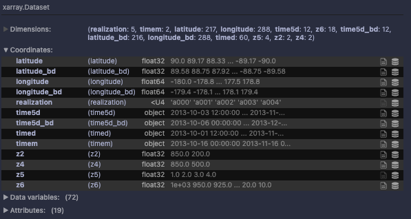
The information content looks like this: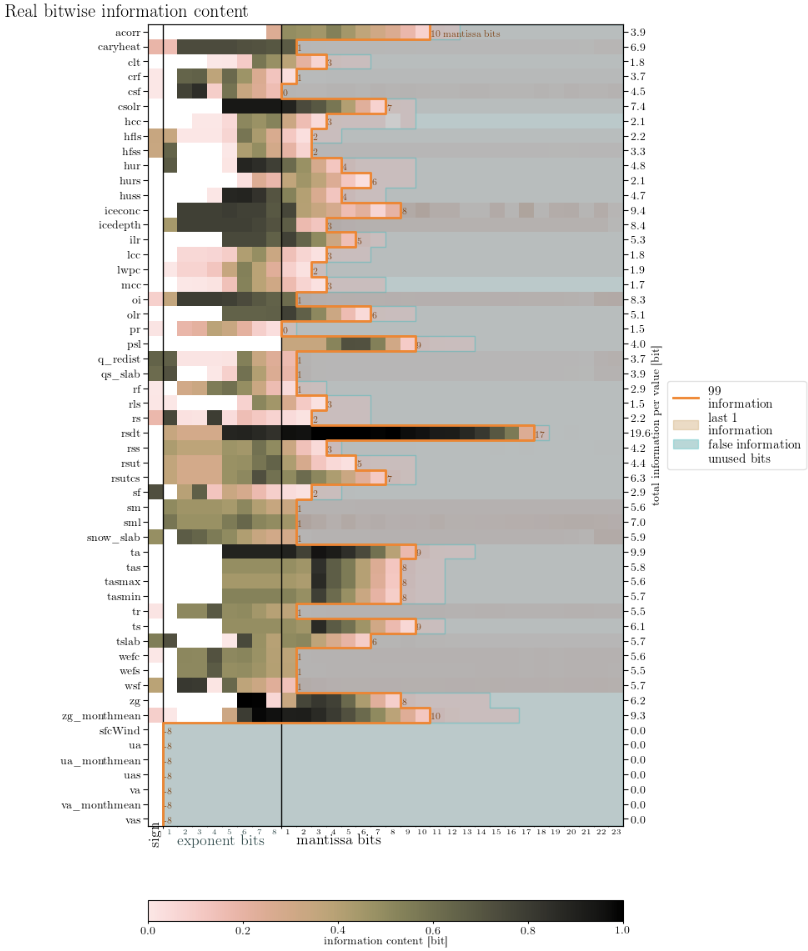
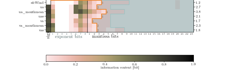 (had to be done in two steps - different longitude coordinates)
By default, precipitation is saved in kg/m^2/s, with goes from zero (plus a few negative points) to 1e-3. Following the basic pipeline led to compressed precipitation looked quite a bit different (more clunky, like a filled colour plot) than the uncompressed: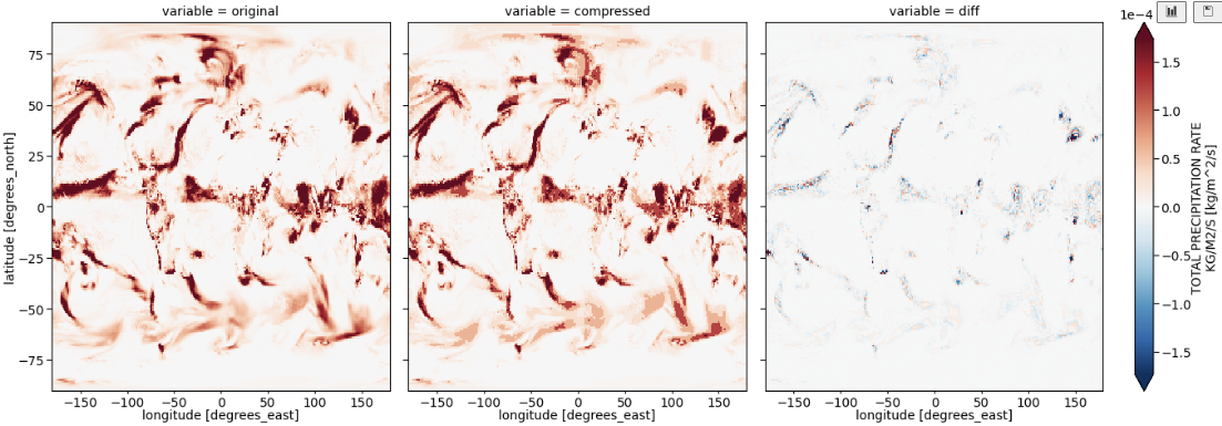
Physically, I prefer precipitation instead in mm/day, involving multiplying by a factor of 86400. I've done a bit of experimenting with converting the data to float64 and/or multiplying with a factor (as int -> data becomes float64; as float -> data stays float32), which yields quite different results in how many bits the algorithm likes to keep: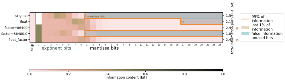
I was wondering if you had some insights. For example
I also did a bit of testing of saving the tutorial (https://xbitinfo.readthedocs.io/en/latest/quick-start.html) as .nc and .zarr. I noticed that while for netcdf, the file size decreases with "better" compression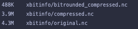 this is not the case with zarr, where weirdly the uncompressed is smallest, the initial compression increases the size, and the the rounded compression is smaller, but almost a factor of 2 larger than netcdf.
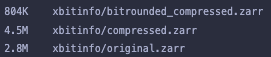
Did you find this too, and do you have an explanation?
Thanks! Matthias