How to replicate the circle trajectories like README.md

20chase commented 5 years ago

Hi Michael,

Thanks for your great jobs.

I am running this repo on Stage simulator, while the circle trajectories are not like the figure in README.md.

Here is the trajectory I run in Stage.

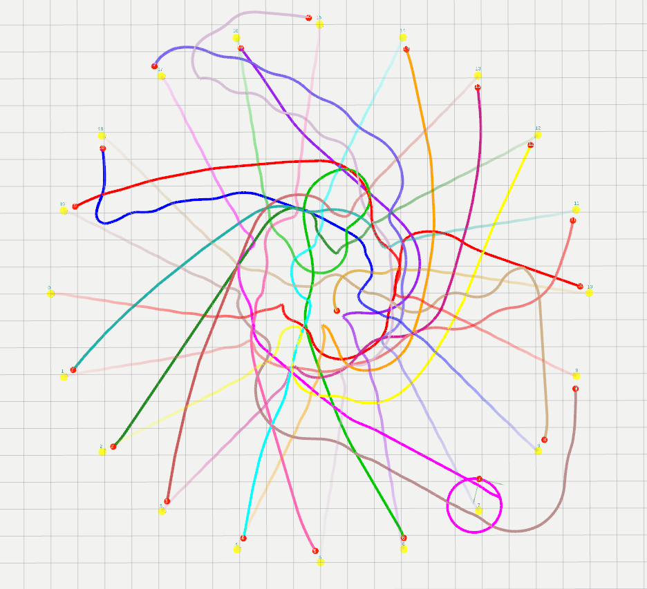
Some parameters of my experiments as follows:

the radius of the circle scenarios: 10.0
the radius of robots: 0.36
the maximum velocity: 1m/s for linear velocity, 1/rad for angular velocity
differential drive platform
load model: 01900000
not noise

The code details:

        """
        poses:
            all pose information of robots in the global coordinate system
            poses[i, 0]: the ith robot position at the x-axis
            poses[i, 1]: the ith robot position at the y-axis
            poses[i, 2]: the ith robot heading angle

        goals:
            all goal position information in the global coordinate system
            goals[i, 0]: the goal position of the ith robot at the x-axis
            goals[i, 1]: the goal position of the ith robot at the y-axis

        self.radius:
            the radius of all robots (0.36m)

        self.max_vx:
            the maximum velocity of all robots (1m/s)

        global_vels:
            the velocity information of all robots in the global coordinate system
            global_vels[i, 0]: the velocity of the ith robot at the x-axis
            global_vels[i, 1]: the velocity of the ith robot at the y-axis

        """
        obs_inputs = []
        for i in range(self.num_agents):
            robot = Agent(poses[i, 0], poses[i, 1], 
                          goals[i, 0], goals[i, 1], 
                          self.radius, self.max_vx, 
                          poses[i, 2], 0
                          )
            robot.vel_global_frame = np.array([global_vels[i, 0],
                                               global_vels[i, 1]])
            other_agents = []

            index = 1
            for j in range(len(poses)):
                if i == j:
                    continue

                other_agents.append(
                    Agent(poses[j, 0], poses[j, 1],
                          goals[j, 0], goals[j, 1], 
                          self.radius, self.max_vx,
                          poses[j, 2], index 
                         )
                )
                index += 1

            obs_inputs.append(
                robot.observe(other_agents)[1:]
            )

        actions = []
        predictions = self.nn.predict_p(obs_inputs, None)
        for i, p in enumerate(predictions):
            raw_action = self.possible_actions.actions[np.argmax(p)]

            actions.append(np.array([raw_action[0], raw_action[1]]))

Do I misunderstand the code or wrongly set the parameter?

Looking forward to your reply : )

mfe7 commented 5 years ago

a couple thoughts:

how often are the agent actions being updated? the training occurs at dt=0.2sec but in our experiments we use dt=0.1 for execution, which leads to much better performance.

what is the model for robot dynamics? in training, our agents set their heading angle and velocity directly, so any extra acceleration-type constraints would cause the policy to be less useful.

the agents were trained in crowds of up to 10 agents, but we saw good results in a few 20-agent setups. i wouldn't expect it be super reliable in generic 20-agent cases, especially if the simulator isn't quite like the one from training.

the lack of symmetry is puzzling, since all agents should be moving identically and receiving identical observations (assuming they started in the same states). any idea if there is something in your simulation that would lead to asymmetric network inputs?

20chase commented 5 years ago

Hi Michael,

Thanks for your kind reply. The frequency of the execution is 10hz and any dynamics constraint didn't be introduced.

The problem is that the observations for the RNN input computed by the observe function in the agent class have different order although the position and velocity information is symmetry. In this case, the RNN will output different commands for them. Here is a simple example.

agent_num 0 obs: 
[ 2.   10.   -0.    1.    0.36  2.5   4.33  0.    0.    0.36  0.72  4.28
  2.5  -4.33  0.    0.    0.36  0.72  4.28  0.    0.    0.    0.    0.
  0.    0.    0.    0.    0.    0.    0.    0.    0.    0.    0.    0.
  0.    0.    0.    0.    0.    0.    0.    0.    0.    0.    0.    0.
  0.    0.    0.    0.    0.    0.    0.    0.    0.    0.    0.    0.
  0.    0.    0.    0.    0.    0.    0.    0.    0.    0.    0.    0.
  0.    0.    0.  ]
agent_num 1 obs: 
[ 2.   10.    0.    1.    0.36  2.5  -4.33  0.    0.    0.36  0.72  4.28
  2.5   4.33  0.    0.    0.36  0.72  4.28  0.    0.    0.    0.    0.
  0.    0.    0.    0.    0.    0.    0.    0.    0.    0.    0.    0.
  0.    0.    0.    0.    0.    0.    0.    0.    0.    0.    0.    0.
  0.    0.    0.    0.    0.    0.    0.    0.    0.    0.    0.    0.
  0.    0.    0.    0.    0.    0.    0.    0.    0.    0.    0.    0.
  0.    0.    0.  ]
agent_num 2 obs: 
[ 2.   10.    0.    1.    0.36  2.5   4.33  0.    0.    0.36  0.72  4.28
  2.5  -4.33  0.    0.    0.36  0.72  4.28  0.    0.    0.    0.    0.
  0.    0.    0.    0.    0.    0.    0.    0.    0.    0.    0.    0.
  0.    0.    0.    0.    0.    0.    0.    0.    0.    0.    0.    0.
  0.    0.    0.    0.    0.    0.    0.    0.    0.    0.    0.    0.
  0.    0.    0.    0.    0.    0.    0.    0.    0.    0.    0.    0.
  0.    0.    0.  ]
agent_num 3 obs: 
[ 2.   10.    0.    1.    0.36  2.5   4.33  0.    0.    0.36  0.72  4.28
  2.5  -4.33  0.    0.    0.36  0.72  4.28  0.    0.    0.    0.    0.
  0.    0.    0.    0.    0.    0.    0.    0.    0.    0.    0.    0.
  0.    0.    0.    0.    0.    0.    0.    0.    0.    0.    0.    0.
  0.    0.    0.    0.    0.    0.    0.    0.    0.    0.    0.    0.
  0.    0.    0.    0.    0.    0.    0.    0.    0.    0.    0.    0.
  0.    0.    0.  ]
agent_num 4 obs: 
[ 2.   10.   -0.    1.    0.36  2.5  -4.33  0.    0.    0.36  0.72  4.28
  2.5   4.33  0.    0.    0.36  0.72  4.28  0.    0.    0.    0.    0.
  0.    0.    0.    0.    0.    0.    0.    0.    0.    0.    0.    0.
  0.    0.    0.    0.    0.    0.    0.    0.    0.    0.    0.    0.
  0.    0.    0.    0.    0.    0.    0.    0.    0.    0.    0.    0.
  0.    0.    0.    0.    0.    0.    0.    0.    0.    0.    0.    0.
  0.    0.    0.  ]
agent_num 5 obs: 
[ 2.   10.   -0.    1.    0.36  2.5   4.33  0.    0.    0.36  0.72  4.28
  2.5  -4.33  0.    0.    0.36  0.72  4.28  0.    0.    0.    0.    0.
  0.    0.    0.    0.    0.    0.    0.    0.    0.    0.    0.    0.
  0.    0.    0.    0.    0.    0.    0.    0.    0.    0.    0.    0.
  0.    0.    0.    0.    0.    0.    0.    0.    0.    0.    0.    0.
  0.    0.    0.    0.    0.    0.    0.    0.    0.    0.    0.    0.
  0.    0.    0.  ]
==> poses: 
[[ 5.     0.    -3.142]
 [ 2.5    4.33  -2.094]
 [-2.5    4.33  -1.047]
 [-5.     0.    -0.   ]
 [-2.5   -4.33   1.047]
 [ 2.5   -4.33   2.094]]
==> action: 
[array([1.        , 0.26179939]), array([1., 0.]), array([1.        , 0.26179939]), array([1.        , 0.26179939]), array([1., 0.]), array([1.        , 0.26179939])]

After "unifying" the input, the trajectory can be plotted as below:

mfe7 commented 4 years ago

@20chase not sure if still useful, but looking at this the agent sizes seem quite small in the picture, so maybe they are outside the range it was trained on (i think 0.2-0.8m radius if i remember correctly?). also your observations only have a couple agents in them - with that many agents the observation vector should be quite dense.

mit-acl / cadrl_ros

How to replicate the circle trajectories like README.md #7