Building qualification using baseline model fit

[hshaban]

Buildings with usage patterns that are not correctly captured using Caltrack models end up with low signal-to-noise ratio, poor model fits and tend to default to the intercept-only model. These buildings are not suitable for Caltrack/regression modeling and are recommended to be handled using alternate methods.

We propose the following:

1. Identify metrics to determine the suitability of the Caltrack baseline model for calculating payable savings.
2. Variance of monthly or daily usage on intercept-only models relative to mean usage be used to judge the quality of intercept-only models (in lieu of R-squared)

[jskromer]

A low signal to noise ration (high CVrmse) can be caused by randomness in the signal at times that are not particularly relevant to the retrofit. For example, what if the expected savings are all happening during the occupied hours (weekday). Any noise on the weekends could be ignored. Applying a strategy of removing noise this way would require a good ex-ante load shape model. And that's probably a good topic for another issue.

[mcgeeyoung]

@jskromer One question we are exploring is whether CVRMSE is the appropriate metric for evaluating the baseline. It's certainly conventional wisdom, but what RMSE actually measures is different than what we are thinking matters. That is, the question of stability of the baseline when an intercept model is used requires us to look outside CVRMSE at something like Mean Absolute Error or MAPE. But we certainly want to test this question extensively.

[hshaban]

One thought from @danrubado on how to handle poor weather model fits:

There may also be an R-squared floor for candidate weather models, below which the "intercept-only" model is selected. We have used R-squared < 0.5 as a floor for candidate weather models in the past.

[hshaban]

Preliminary questions regarding building qualification:

• Should we accept intercept only models? What's a good metric to assess an intercept-only model fit?
• How do our metrics and methods align with pay-for-performance programs? Do they reflect performance risk and uncertainty? Are they convenient for implementers and aggregators?
• What should we do with disqualified buildings? Are they eliminated from participating in pay-for-performance programs or is there another way to accommodate them?
• What metrics and thresholds are useful for assessing baseline model fit in a pay-for-performance context?

[steevschmidt]

There are many homes in California with very small heating and cooling loads. I do not know how CalTRACK methods will treat these homes, but often they have the best opportunities for low-cost savings and should not be excluded from P4P programs.

Two examples below (one high energy, one low energy). These charts show a year of disaggregated energy use, including both electricity and natural gas, shown in cost per month. Note the small percentages of heating (red) and cooling (light blue) energy.

High energy:

Low energy:

[hshaban]

Thanks for the examples, @steevschmidt. I think the challenge with intercept-only models is determining when the intercept coefficient represents a baseload and small heating/cooling loads vs. when it's just an average of noisy data. The examples you posted above will probably be fit with a qualified Caltrack model, but the following building will get a fit as well. This one looks suspiciously like a vacation home, so might need some custom analysis. What we're looking for in this task is a way to distinguish between stable buildings like the ones you posted (which can use the default Caltrack methods) and buildings like the one below where the default Caltrack models are not suitable, so they should be flagged for an alternate/custom analysis route.

[steevschmidt]

I'd be pretty surprised if your green chart above is from a real home: several months show zero electric use, and most people don't unplug their fridge or other plug loads when they go on vacation. Below is a more realistic example of a long vacation:

[hshaban]

:-) Funnily enough it is from a real building, although I'm not sure what the correct interpretation is yet (maybe intermittent meter failures?). It's definitely a very extreme case, but that's still the idea: when should we take a closer look at model fits? Is there a metric that tells us the model for the building you just posted above needs some adjustment?

[rsridge]

Here are some thoughts to two of the homework questions:

• What do we use to eliminate models? R-square? CVRMSEP MAPE? • Any literature to recommend? Why CVRMSE?

Here some references regarding root mean squared error (RMSE), MAPE and others:

1. Kennedy, peter. (2008). A Guide to Econometrics. Malden, MA: BLACKWELL PUBLISHING (p.334).
2. Baum, Christopher F. An Introduction to Modern Econometrics Using Stata. College Station, TX: Stata Press. (p. 69)

However, my brief review indicates that the standard statistical references do not address the coefficient of variation of the root mean Squared Error (CVRMSE). Here three references that do address it.

3. https://stats.idre.ucla.edu/other/mult-pkg/faq/general/faq-what-is-the-coefficient-of-variation/ (accessed March 5, 2018).
4. Efficiency Valuation Organization. (2012). International Performance Measurement and Verification Protocol: Concepts and Options for Determining Energy and Water Savings: Volume 1 (p. 96)
5. Overview of ASHRAE Guideline 14-2002 : Measurement of Energy and Demand Impacts (http://www.managingenergy.com/~managi5/images/pdf/managingenergy_ashrae_guideline_14.pdf)

Only the UCLA document discusses its advantages while only the ASHRAE Guideline suggests criteria for selection, one for energy (<20%) and one for demand (<30%).

[goldenmatt]

It seems like in general there are always outliers... homes that use $300 in baseload but essentially nothing in HVAC - leads me to think there is something going on that we are not seeing in the data. Similar to my own home, where I have heating usage in the summer because I am actually on the north side of a hill and bedrooms are just cold even in the summer - at least for now (I'm working on my retrofit). I think while we want to handle outliers, there are limits to modeling these bizarre circumstances - which of course or more common on "broken" buildings (the very ones we want to focus on).

Steve, do you have the fuel consumption data behind your end use models?

[steevschmidt]

Steve, do you have the fuel consumption data behind your end use models?

Yes, of course. Difficult to share tho. I have been assuming that CalTRACK supports condos and apartments too... is that not the case? Because many of them have very low HVAC energy use.

[goldenmatt]

Well, there is nothing to assume, the CalTRACK 1.0 model selection process is documented here: https://goo.gl/kiGmpJ

The model selection process would simply use an intercept model when there is not an acceptable HDD or CDD model fit.

If you wanted to test these houses on the CalTRACK model you can always use the web version of the OpenEEmeter which runs the methods: https://webopeneemeter.openee.io/

[bkoran]

Regarding the use of MAPE vs. CV(RMSE): It seems they would have equivalent utility for monthly models, but not at all for daily or hourly models, at least as I have seen it defined from LBNL, which uses monthly MAPE.

[mcgeeyoung]

Good point. In my original thinking on this issue, I had mostly been considering monthly irregularity as the defining feature of a quality baseline. I'll see about putting this into a slide for tomorrow, but the goal is to qualify a project with an intercept-only baseline model. If the usage is stable (this could be daily or monthly, really), and it drops after the intervention, I think we'd be more likely to accept the savings than if the usage is highly erratic in the baseline period and then, on average, drops in the reporting period. My understanding of CVRMSE is that it minimizes the effects of outliers, which may not be the side that we'd want to err on (then again, maybe it is!). I'm hopeful that we can come up with an empirically tested number that we can use to discern a reasonably stable baseline.

[bkoran]

Like I just wrote on another topic, I use the t-statistic of the slope of a time-series of residuals to test baseline stability, but this gets into issues of seasonality etc. that I covered on the other topic.

[mcgeeyoung]

Yeah, we need to avoid the Turtles all the way Down problem when getting into these things.

[steevschmidt]

I mentioned this case in the call today: a home assigned to CalTRACK's intercept_only model due to noise from EV charging: We have reason to believe this home used over 1200 kWh for heating over the past 12 months. But because the intercept_only model was assigned, this portion of electric use will not be weather-normalized in CalTRACK. This could result in significant errors when calculating savings... depending entirely on the specific weather changes between baseline and reporting periods: savings could be under- or over-reported. Over a large pool of homes this might wash out, as Hassan pointed out during the call.

However, there appears to be a systemic problem: if the weather is extreme during the base year, there's more obvious correlation between weather and energy, and the chances of assigning intercept-only models decrease (which is good for everyone). But if the weather is mild during the base year there will be more intercept-only models assigned.... and then when the reporting year has more weather (even average weather), the intercept-only model will report this as increases in energy use -- not the result of weather. This systemic imbalance would be bad for P4P aggregators.

The alternative of excluding this home seems like a bad approach, given the growth of EVs.

[CBestbadger]

Here is the paper that Steve Kromer had noted in the meeting on Thursday: Southern California Edison with FirstFuel. February 2016. Energy Efficiency Impact Study for the Preferred Resources Pilot with the four building classification.

[CBestbadger]

Similarly - this study done by Jessica Granderson et. al. considers issues of pre-screening: Granderson, J., Price, P., Jump, D., Addy, N., Sohn, M. 2015. Automated Measurement and Verification: Performance of Public Domain WholeBuilding Electric Baseline Models. Applied Energy 144:106-133.

[steevschmidt]

From the weekly CalTRACK Methods update:

Intercept-only models imply no significant effect of HDD or CDD on energy consumption was detected. Generally, this means that weather did not have a significant effect on the site’s energy consumption.

I suggest this text would be more accurate as follows: "Generally, this means weather related effect on the site’s energy consumption was not detected by CalTRACK algorithms."

The reason this correction is perhaps significant --

If a mild weather year (the baseline period) for a home with lots of energy noise prevents a clear regression to temperature, and this year is followed by a more extreme weather year (the reporting period), the weather-related energy use in the home will of course increase.

The weather-related energy use in the reporting period may then be measurable by CalTRACK methods, but since CalTRACK methods assign a model only during the baseline year, this situation would [systemically] result in these homes looking like they increased their energy use (the opposite of savings) when in fact the energy use may have been proportional to the weather change and real savings may have occurred.

The opposite case of an extreme weather year followed by a mild weather year would not have this problem, since an HDD or CDD model would be assigned during the baseline period and used again during the mild weather year.

This appears to be a case where the assignment of an "intercept-only" model could systemically penalize aggregators.

I cannot propose a specific solution to this problem; I only raise the issue for consideration, along with the assertion that most building do have real heating and cooling loads... whether or not CalTRACK methods can identify them.

[margaretsheridan]

Here is a repost of some distributions of adjusted R squared and CVRMSE for around 500,000 SMUD customers. I broke them out by residential vintage and commercial size. This is a starting point for getting a better understanding of the predictability of loads. More to come later... ResCommHistograms.docx

[bkoran]

@margaretsheridan, that is great information. I get to see many individual building models, but not very large numbers of individual models, with summaries like this. The charts for SMB and non SMB CI are very encouraging, but not surprising. (I suspect not too many industrial were included, and some of them were likely the outliers on the histogram.) The TOWT model is a very good model in most cases for these purposes. It would be helpful to see CV(RMSE) with a scale more focused on the majority of sites.

[steevschmidt]

Thanks for the great data Margaret! We work only on residential, and I'm struck by the huge difference in quality of fit between res and non-res shown in your charts... do you have a working hypothesis for this?

[bkoran]

Not requested of me, but FWIW my opinion is that commercial has much more consistent schedules of people and operations, and likely much less changing of heating and cooling setpoints. On the other hand residential models work very well with aggregates; I suspect commercial less so unless very careful segmentation is used.

[margaretsheridan]

I see a large amount of variability in the commercial and industrial meter data (i.e. a data center with very high R squared vs a construction company with very low R squared). This variation then translates to the consistency of the statistical predictability of the load. There is also considerable churn with normal business operations transitioning to vacancies or entirely different load shapes as one business replaces another at the same location. Some of these details can be worked out of the data by including billing information. These distributions represent the first raw cut at the populations.

[bkoran]

I have multiple comments on this subject:

Related to the concept of weather temperature ranges changing from baseline to post is "coverage factor." This relates to @steevschmidt 's comment regarding the change in weather from baseline to post. The Guidance for Program Level M&V Plans: Normalized Metered Energy Consumption Savings Estimation in Commercial Buildings draft includes a brief mention of coverage factor. Other guidance by David Jump and others includes a time-related component to coverage factor.

Also, there is an implicit assumption that only forecast models will be used, and never backcast models. For these types of situations, backcasting may be preferable. For electricity use in CA, it will seldom be necessary, but for gas use it could be needed more often.

The whole concept of "

[bkoran]

The whole concept of "Building qualification using baseline model fit" cannot be separated from the model used. For example, the TOWT model, when used in an automated fashion, can exclude the definition of daytypes. This can result in poorer model fits than if daytypes were defined.
(The TOWT model uses a temperature relationship developed for all hours of the week, and then has coefficients for each hour of the week to provide an offset for each hour from the model of all hours. Therefore, it does not necessarily model the temperature relationships accurately for each hour, just overall. The TOWT model in the Universal Translator allows the user to define daytypes.)

In CalTRACK 2.0, the definition and use of daytypes (and 'hourtypes') is TBD. Very misleading results can occur if daytypes are not defined. An office building that is open just 5 days per week, and shuts down extremely well on weekends, with significant HVAC setbacks, can have a poorer fit than a building that is just moderately consistent but operates 7 days per week, if separate models for weekdays and weekends are not included.

A similar situation can occur with hourtypes. Note that change points/base temperatures are not constant during the day, but are usually different between occupied and unoccupied periods. When we need to know the timing of savings, which should be important, we probably shouldn't assume the same change points and weather relationships between all hours of the day and all days of the week.

Overall, this gets into model uncertainty. If we are disqualifying buildings, is it because they have inconsistent operation, or because we have an inadequately specified model?

[steevschmidt]

Agree with bkoran: if we are disqualifying a lot of buildings the focus should be on improving the models. I also like the coverage factor and backcasting ideas... perhaps used together as our weather patterns get more extreme.

[mcgeeyoung]

@bkoran wrote "The whole concept of "Building qualification using baseline model fit" cannot be separated from the model used." Actually, that's the point here. We are specifying the model(s) to be used through this process. There should be no discretion, which is what creates uncertainty and prevents markets from stabilizing. If I don't know which model you are going to use until after the project has been completed, I have no way of knowing what my yields are likely to be. Up until now we have been assuming that the model would be daily or based on billing data. The building qualification guidance also reflects this core assumption. However, once we get into hourly models, we'll want to revisit these assumptions around r2 and cvrmse (and probably others too). I don't at all disagree with your conclusion that we need to understand the difference between model uncertainty and building energy consumption inconsistency. But what we're trying to do here is hold the model constant and understand its limitations with respect to different types of modeling challenges. Once we introduce hourly methods, it will probably be important from the outset to specify the particular model that is being used in order to determine the relevant qualification criteria. Let's make sure to pick that back up at the appropriate time.

[bkoran]

@mcgeeyoung wrote "Actually, that's the point here. We are specifying the model(s) to be used through this process. There should be no discretion, which is what creates uncertainty and prevents markets from stabilizing. "

I don't disagree, and understand that is the point. However, this is not just an issue for hourly models, but also for daily models. How the models will handle daytyping has not been specified, or if they have I have missed it, and this is being discussed in https://github.com/CalTRACK-2/caltrack/issues/83.

So we are attempting to create criteria for building exclusion, without knowing the quality of the models that will be doing the exclusion. As a believer in these methods, I don't want to see buildings excluded because models are inadequately specified, when the buildings themselves might have very consistent operation that can be well modeled with appropriate specification.

[steevschmidt]

Again I agree with bkoran, and I think we're just pointing out there needs to be a process for continuous improvement of CalTRACK methods. They can't be "cast in concrete", especially at this early stage.

[bkoran]

@steevschmidt said the important thing that I didn't say at all: We need to have continuous improvement, or at least accept some interation. If we set criteria now, they should probably be revisited after models are set.

[mcgeeyoung]

I think we all kind of want the same thing here. Consistency, improvement, specificity. At a general level, CalTRACK creates consistency; the CalTRACK process allows for ongoing improvement; the testing and discussion around the methods creates the specificity. I would hope that as we make progress, we continually reflect on our basic assumptions and adapt them. For example, monthly methods started out with a fixed balance point temperature. Now we're agreed to allow for a search grid. The evidence points to this being an improvement in the quality of the savings calculation. And if someone is following the methods specified by CalTRACK 2.0 for analyzing billing data, we can be confident that they are following the temperature set point rules, which where the specificity comes in. I know it's a bit frustrating to be working in such an incremental fashion, but in the long run we will really benefit from being so diligent.

[hshaban]

Results discussed on the March 29th call:

The model-fit metrics

The metrics used to evaluate model fit in this task are defined below:

The Coefficient of Variation of Root Mean Squared Error (CVRMSE) is simply the root mean squared error of the model divided by the mean energy usage.

The Mean Absolute Percent Error (MAPE) is calculated by taking the overall mean of the individual absolute percent error for each individual data point.

The Normalized Mean Absolute Error (NMAE) is calculated by taking the mean of the individual absolute errors for each individual data point, then dividing by the mean energy usage to express the MAE as a percent.

CVRMSE is a commonly used metric in M&V guidelines, such as ASHRAE Guideline 14 and the Uniform Methods Project. However, squaring errors tends to exaggerate the effect of outliers (i.e. it increases with the variance of the individual errors). This is apparent when comparing it to NMAE in Figure 1. Across all building types, CVRMSE appears to follow the same trends as NMAE, but its distribution is wider, with fatter tails. Therefore the choice between these two metrics will come down to whether it is desirable to have an additional penalty on individual predictions that have large errors (CVRMSE) vs. penalizing all errors equally regardless of their magnitude (NMAE).

The MAPE, on the other hand, appears very similar to the CVRMSE for most building types, except for colleges, schools and agricultural facilities, where the MAPE becomes visibly larger than the CVRMSE distribution. This is because MAPE penalizes data points with small usage values yi. These three building types have highly seasonal usage, meaning that during certain times of the year, the energy use diminishes significantly. Models that are wrong during these periods of time would be more heavily penalized by the MAPE metric because the percent errors grow with smaller yi, whereas, the absolute errors on the lower end of the spectrum are bounded, so CVRMSE and NMAE are not as affected (e.g. a single data point where the usage was close to zero would push MAPE towards infinity).

Figure 1. Comparison of different model-fit metrics for intercept-only models in commercial buildings.

Commercial building types

Figure 2 illustrates the distribution of annual energy use vs. model fit (CVRMSE) for various building types. The size of the bubble indicates the number of meters for each building type and can be thought of as a proxy for a technically achievable portfolio size. Building types with smaller bubbles may not benefit from the uncertainty-reduction advantages of lumping assets into portfolios.

The chart is also divided into 3 regions, the boundaries of which are illustrative and by no means set in stone. Region A (lower left) includes building types for which the average CVRMSE falls within the 20-40% range (as a point of reference, ASHRAE Guideline 14 recommends a CVRMSE of 25% or less for baseline models). The annual energy usage of these buildings is also on the lower end of the spectrum, making them more amenable to whole building energy modeling. With some updates to certain CalTRACK parameters, these building types could probably be successfully modeled within reasonable tolerance (especialy those included in the Monthly and Daily Methods updates). Region B (lower right) includes building types with very high annual energy use, CVRMSE close to 40% and small portfolio sizes. Colleges, hospitals and industrial facilities also generally consist of several buildings and each building might be mixed-use, so unless submetering is implemented and other independent variables are included in the analysis, it would be extremely difficult to detect the energy use changes that would result from most energy efficiency interventions. Finally, Region C includes high-CVRMSE building types, where effects other than weather likely dominate the energy use and current CalTRACK models will likely be insufficient for modeling, especially with the availability of only billing data.

Figure 2. Energy use vs. model fit characteristic diagram. Building types in region A are potential candidates for CalTRACK modeling, region B may require submetering and region C require additional independent variables.

CVRMSE thresholds

Developing guidelines for CVRMSE cutoffs is difficult because different datasets may have different distributions of model quality (depending on sector, building type, data granularity, location etc.). Moreover, for pay-for-performance, the major concern is portfolio performance and uncertainty rather than individual model fit. Figures 3 and 4 demonstrate the attrition experienced by different portfolios, when different CVRMSE thresholds are implemented at the building level. In general, very little attrition happens with large thresholds (>1), with incremental improvements in both portfolio performance metrics. With thresholds below about 0.6-0.8, attrition is much higher (e.g. 40% of the portfolio could be ineligible with a 25% CVRMSE threshold). However, the incremental reduction in portfolio uncertainty is minimal at best, especially for the larger portfolios. Smaller portfolios generally have larger portfolio-level uncertainty, and in some cases, are susceptible to the influence of outliers on the portfolio-level uncertainty (this is the case with the large drops in portfolio uncertainty at 1.2 and 1.4 CVRMSE cutoffs for office buildings).

While smaller portfolios may benefit from tighter thresholds, there is no way to predict upfront what threshold is suitable for a particular dataset, making guidance on this matter challenging. However, if the goal is to achieve relatively low portfolio-level uncertainty, then it may make sense to specify a large building-level threshold, but limit the acceptable portfolio-level uncertainty. If portfolios do not fall under this acceptable level, then aggregators may choose to either increase the size of the portfolio or eliminate specific buildings using tighter building-level thresholds.

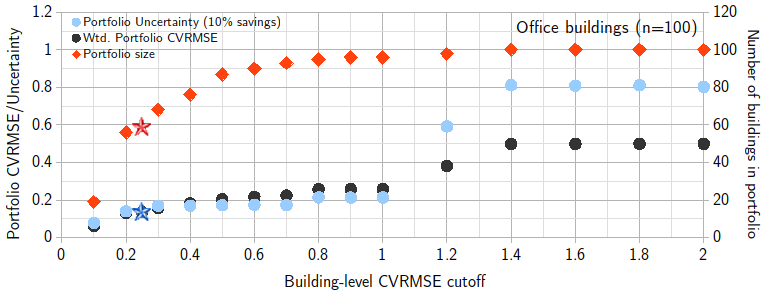
Office buildings Figure 3. Variation of portfolio size, weighted mean CVRMSE and portfolio fractional savings uncertainty with different building-level CVRMSE cutoffs for office buildings. Stars represent the ASHRAE Guideline 14 recommended cutoff (CVRMSE=25%).

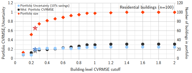
Residential buildings Figure 4. Variation of portfolio size, weighted mean CVRMSE and portfolio fractional savings uncertainty with different building-level CVRMSE cutoffs for residential buildings. Stars represent the ASHRAE Guideline 14 recommended cutoff (CVRMSE=25%).

Recommendations

• We recommend using CVRMSE as the main metric for evaluating baseline model fit for the following reasons:
  • Buildings with outlier energy use significantly affect portfolio savings uncertainty and it is preferable to eliminate them. CVRMSE penalizes such buildings, making it more likely that they are eliminated from the portfolio.
  • CVRMSE is not sensitive to the individual usage values making it more robust than MAPE and similar metrics.
• We are recommending that the specific building eligibility requirements be generally left to the procurer, who can set the requirements that align best with their goals for a procurement, provided these are specified clearly upfront. CalTRACK can provide general guidelines as follows.
  • For use cases where confidence in portfolio-level performance is required (e.g. aggregator-driven pay-for-performance, non-wires alternatives (NWA) procurements), we recommend using a permissive building-level CVRMSE threshold (100% is recommended), but requiring that a portfolio-level metric be respected (e.g. weighted mean CVRMSE or portfolio fractional savings uncertainty). The portfolio-level threshold will be a policy decision and may differ depending on the use case (e.g. NWA procurement may require less than 15% uncertainty, regular pay-for-performance program may require 25% to align with ASHRAE Guideline 14 etc.)
  • For use cases where confidence in individual building results is required (e.g. customer-facing performance based incentives), ASHRAE Guideline 14 thresholds may be used.

[steevschmidt]

To try to get a better handle on the CVRMSE values discussed above, we've been using CalTRACK models with CVRSME around 50% to calculate monthly energy use within the baseline period, and then comparing to actual monthly totals. We see large errors: +/- 50%. Is this expected?

With 30 data points per month, is there a reason CalTRACK did not consider monthly regressions?

[bkoran]

Comments and questions:

I agree with the use of CVRMSE as a main criterion for model evaluation. I strongly urge that the maximum bias be reduced to near zero; I believe the CalTRACK models already meet a much lower bias requirement.

I said this on the call, but I'll repeat my statement that "Moreover, for pay-for-performance, the major concern is portfolio performance and uncertainty rather than individual model fit" is not always true! It depends very much on program design and who receives the performance incentives.

Figure 1: Intercept-only models will have relatively poorer fits for smaller buildings than for larger buildings, because smaller building loads are relatively more impacted by weather.

Figure 2: What models (CalTRACK 1 or 2, intercept only or best choice among available PRISM-type models, monthly or daily?) were used to get the building CVRMSE values?

In general, I am quite surprised at the CVRMSE values for several sectors. I expect much lower than shown for most offices, hospitals, and at least some types of retail, e.g. big box, even for hourly models, which have higher CVRMSE than daily, which have higher CVRMSE than monthly.

Figures 3: Again, What models (CalTRACK 1 or 2, intercept only or best choice among available PRISM-type models, monthly or daily?) were used to get the building CVRMSE values?

[mcgeeyoung]

@steevschmidt Not sure that we even considered monthly regressions. How would that work? In terms of variance from predicted to actual, on any given day you should expect quite a bit of variance - people do laundry, vacuum, etc. You want to look at the whole year.

[mcgeeyoung]

@bkoran I'll let Hassan answer the specific questions about his data. But just wanted to underscore an important principle of CalTRACK (and this set of updates in particular), which is that it's not aiming to cover all use cases out of the gate, but rather is trying to prioritize the particular programmatic objectives of the CEC, PG&E, NYSERDA, Energy Trust, SMUD and other participating procurement organizations. If you were to pay customers directly for their savings, CalTRACK would probably be a poor choice of methods for a variety of reasons, not the least of which would be building qualification criteria. However, the animating principle of the P4P model that CalTRACK is primarily designed to support is that a third party aggregator will be taking on the performance risk and will be contracting with a procurement entity that has to answer to regulators. Thus, the major methodological goals of the CalTRACK process are going to be focused on issues that are at the center of this particular policy structure, even at the expense of other P4P approaches.

[goldenmatt]

I think that getting clear on our terms is really critical to avoid arguing in circles. P4P is a completely overpacked word... it can mean aggregated savings to utilities, it can also mean an ESCo agreement. While many of the same principles apply in both cases, there are some really big differences in how we measure in each case, and both are important. But when you try and achieve both use cases at the same time with the same math, you don't do either justice. I wrote this article a while back on this topic if it helps:

https://www.linkedin.com/pulse/pay-for-performance-energy-efficiency-comes-two-flavors-matt-golden/

[hshaban]

@bkoran Figures 2 and 3 use the best choice among available, Caltrack 1 monthly models. Figure 2 uses much larger samples (tens of thousands of buildings), while Figure 3 starts with a random sample of 1000 buildings. I'll be re-running these buildings with Caltrack 2 at some point, to see if there's a change in the CVRMSE distributions.

To answer a separate question I got this week, the weights in weighted CVRMSE are the mean usage values for each building. So it's equivalent to adding the model RMSE values for all buildings then dividing by the total usage for those buildings. I just used it as an illustration of the CVRMSE for the portfolio (there might be better ways to aggregate CVRMSE), but again, at the portfolio-level, we would care more about the fractional savings uncertainty than CVRMSE.

[bkoran]

Thanks, Hassan.

Matt and McGee, Yes, getting "clear on our terms" and understanding the goals of CalTRACK are very important. I appreciate the reiteration that these savings approaches are not intended to be valid at an individual building level. I have extensive experience with performance contracting, with site-based savings, with implementing M&V, and providing M&V guidance, and well understand the various issues and distinctions.

That said, my point is that the decision-making here pertains to uncertainty. The ways that the terms "CVRMSE" and "uncertainty" have been used has not been clear, and in some cases incorrect. Hassan is working toward making this clear for all of us, and I am trying to help with that. One of my goals is that we don't unnecessarily disqualify buildings as I wrote above. I assume we are all in agreement on that.

[hshaban]

Here's a summary of some on-on-one discussions we've been having with various members of the working group relevant to this topic:

• While CVRMSE is a decent metric for building-level model goodness-of-fit, its values depend on the granularity of data (CVRMSE is generally higher for hourly and daily data). So, applying a single building-level CVRMSE threshold is not appropriate. This is in addition to the variations by building type, location etc. which would make general building-level guidelines very difficult to develop and apply in a consistent manner.

• CVRMSE is not savings uncertainty - CVRMSE is a measure of model fitness and can be used to evaluate how closely a model represents a building's energy use. Fractional savings uncertainty (FSU) is the bounds within which savings are expected to lie (e.g. Savings = 100 kWh +/- 10%). Lower FSU means higher confidence in your results. We are recommending portfolio FSU as the main metric to evaluate portfolio-level results in certain applications. CVRMSE can be used to screen individual buildings prior to an EE intervention, and aggregates of CVRMSE at the portfolio-level may serve as proxies for uncertainty (only the trends, not the actual values). This could be useful in some cases for planning, because calculating FSU requires knowledge of the actual or estimated savings.

• For portfolio applications in particular, aggregating individual building results is a good way to increase confidence in portfolio-level results (reduce FSU). Building-level uncertainties can be aggregated using the square root of the sum of squares, with the assumption that there is no systemic bias in the savings (e.g. stemming from implementation variance, unaccounted for independent variables etc.)

[steevschmidt]

@mcgeeyoung Monthly regressions do a much better job dealing with variable non-HVAC energy use (e.g. behavioral & plug loads), and this type of use now dominate in many homes -- and is growing. Excluding NRAs, energy use still varies from season to season and month to month in most homes. By analyzing at the monthly level, instead of deriving a single intercept plus DD coefficients for the entire year, we get 12 more accurate "models", and individual monthly usage totals match actual energy use for each month.

How would that work?

For savings analysis there are probably many approaches; the one we use it to identify the total heating & cooling loads for the 12 month baseline period along with total HDDs and CDDs, then do the same for a Reporting period of the same duration, which can overlap with the baseline period. We assume a linear relationship between DDs and HVAC energy use, so a simple ratio of DDs between the two periods provides a weather normalization that can be compared to actual use. (This is a high level description; let me know if you need more details.)

...In terms of variance from predicted to actual, on any given day you should expect quite a bit of variance - people do laundry, vacuum, etc....

Sorry if I was confusing: I wasn't talking about daily, just monthly. Since we have 30 data points per month it seems we should use them to more accurately model energy use. (Note this has nothing to do with hourly analysis.) Years ago there may have been a "too compute intensive" argument against doing so, but I think we're well beyond that limitation now.

You want to look at the whole year....

We agree: Seasonal variations matter in many buildings, so it's not good practice to use a single model developed for a full year of energy use to forecast use for some portion of a year, and then measure savings based on it. I could be wrong, but I believe CalTRACK methods currently do this for buildings with less than 12 months post-intervention data.

[mcgeeyoung]

@steevschmidt

We assume a linear relationship between DDs and HVAC energy use

How do you select a balance point and determine the slope?

[mcgeeyoung]

@steevschmidt

then do the same for a Reporting period of the same duration, which can overlap with the baseline period Assuming you mean overlap on a shoulder month (or summer if talking HDD). The underlying premise is that we're doing pre/post savings calcs still, right?

[steevschmidt]

@mcgeeyoung wrote:

How do you select a balance point and determine the slope?

HEA attempted to use correlation-based and R-squared-based balance temperature selection approaches similar to CalTRACK's in early versions of our system but results were poor: energy coaches and homeowners saw that results were not accurate, often resulting in balance point temperatures that were obviously too low.

One possible explanation: The number of daily non-zero HDD data points decreases as the balance temperature drops. The fewer data points the higher R-squared value can be achieved (in the extreme case, there is no difference between model and actual data in the case of just two data points). Because of this relationship between temperature an DDs, the R-squared approach to balance point selection tends to select lower balance temperatures.

Currently we use an average temperature vs average energy usage curve to identify the inflection point(s), which presumably correspond to the balance temperatures when the heating (or cooling) system is turned on. This method is also not ideal because some homes do not have clearly identifiable inflection points, but we have used it for years on thousands of homes and in most cases we are satisfied with the results. It is significantly better than the R-squared approach.

Assuming you mean overlap on a shoulder month (or summer if talking HDD).

No, any overlap between the baseline and reporting period is ok. As long as both periods cover a full 12 months, even 11 months of overlap is ok using this approach. In effect the overlap cancels out, and you are left with the difference in that one new month. This method takes into account a wide variety of monthly (e.g. December holiday lights) and seasonal (e.g. additional summer pool pump run times) variations that are not addressed with a single annual energy model.

The underlying premise is that we're doing pre/post savings calcs still, right?

Correct. We're doing PRISM-like regressions to determine the dependent loads in every month. We sum all load types (e.g. base, cooling, heating) for each of the two 12 month periods. We adjust [only] the dependent loads of the baseline period to the reporting period, using ratios of the independent variables (in our case, CDDs and HDDs, but others are possible). Then we compare the adjusted baseline to the reporting period to determine savings.

I think most of this is very similar to CalTRACK methods, but we are doing it monthly because of the additional data: when there are only 12 data points per year, a yearly model is the best you can do; here we have 365.

[mcgeeyoung]

Interesting. Thanks for explaining @steevschmidt . I'd be interested in hearing what folks with a bit more experience think of this. How do your out of sample tests compare with running the same data through CalTRACK? @bkoran @rsridge @margaretsheridan

[steevschmidt]

@mcgeeyoung wrote:

How do your out of sample tests compare...

Help me understand how out of sample testing is relevant to the specific issue where the model from a baseline year poorly predicts many individual month's energy use within that same baseline year, for that same building? I'd think the accuracy of this "in sample" prediction is more meaningful than out of sample testing, can be easily checked, and could help inform enhancements to the CalTRACK methods.

[mcgeeyoung]

These are two separate metrics, both valuable in their own way. The question of where the model from a baseline year poorly predicts many individual months (or days) energy use within the same baseline year is captured by CVRMSE, MAPE, or NMAE. In our presentation last week, we discussed why CVRMSE offered the most conservative estimate of model error, in that it amplifies the effects of outliers. The higher the CVRMSE, the worse the model predicts any individual month within the baseline period. (It would be a good idea to review the concept of root mean square error if this doesn't make sense from a statistical point of view).

An out of sample test serves a different purpose. Because energy efficiency is a counterfactual, the question you are fundamentally asking is what would the energy use in a building have been if there had been no intervention? One tool we have at our disposal is the ability to study a non-treated group. To the extent that the non-treated group's changing energy use is well-predicted by a model, we are increasingly confident that our model is capturing the causal variables and isolating them so that when we calculate the energy use in a building pre/post retrofit, we are in fact capturing the effects of the intervention.

There are several ways of conducting an out of sample test. The convention in the energy efficiency industry is to examine future participants (taking the two years of pre-treatment data, using the first year as a baseline, and the second year as a reporting period). I don't know why this is the norm, probably a legacy of monthly data and some evaluation-specific criteria. But as long as you have daily data, you could also conduct an out of sample test be removing some subset of your baseline period, fitting a model to the remaining data, and then using the removed data to test how well your model performs. Ultimately, the way that your out of sample test is done is less relevant than the value it provides as an indicator of how well your model performs.

So, when you provide an alternative, and somewhat unorthodox method for calculating savings, it's reasonable to ask how well that model hews to known changes in consumption compared to how other models fare. If you're not familiar with it, I'd highly encourage you to take a look at the work that Jessica Granderson and others at LBNL have been doing comparing different M&V tools. It's very much along these same lines.

And just to reiterate, the goal of CalTRACK is to specify a set of methods that provide a repeatable, transparent, and scalable way to calculate savings across a broad range of buildings and measures. There are a litany of methods for calculating energy efficiency savings that work "better" for particular edge cases. While it's tempting to try to create special rules for all of the different scenarios that arise, the goal of this process is to arrive at a generalized approach that can be used in a uniform fashion to scale pay for performance.

[bkoran]

@mcgeeyoung that was a really great, concise, well-written summary of out-of-sample testing in this arena. It prompted me to share some work of mine that you, @steevschmidt, and others might find of interest. I used a bootstrap and block bootstrap for "out-of-sample" testing for uncertainty, using within sample data, such as you mentioned above for daily data.

IEPEC paper: http://www.iepec.org/2017-proceedings/65243-iepec-1.3717521/t001-1.3718144/f001-1.3718145/a006-1.3718214/an025-1.3718216.html

That IEPEC paper was developed from a larger report I prepared for BPA.

hmm... I apparently did something wrong with the link, but if you copy and paste the URL you'll get to the documents.

One other comment: I don't know if it "The convention in the energy efficiency industry is to examine future participants (taking the two years of pre-treatment data, using the first year as a baseline, and the second year as a reporting period)." That was true of one study done by LBNL and others, but I don't consider it necessarily the convention. I'd be interested in hearing of studies by others that used that approach. To me, it confounds 2 issues: out-of-sample testing and changes in buildings over time. I prefer separating those 2 issues. Both are important, but combining them in a study doesn't provide as much information as looking at them separately.