 steevschmidt
commented
6 years ago
steevschmidt
commented
6 years ago Perhaps related, and just fyi: We did a "Duck Chart" of electric energy efficiency savings results for a program we ran in Mountain View back in 2012. Chart showing results:
 This type of analysis is very easy to do after a program has been completed.
Clarifying 6/7/18: This data is NOT weather-normalized in any way: it is raw smart meter data. Identifying which hours should be weather normalized and by how much is not something we are able to do; to do this we'd have to know which hourly load was the AC unit (which should be normalized) vs the EV charger or pool pump (both of which should not).


 eliotcrowe
 mcgeeyoung
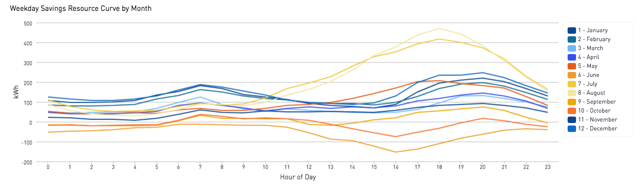
 hshaban

 bkoran
Purpose of this task is to test and recommend methods that can handle hourly data and yield hourly results.