 ldoyle
commented
2 years ago
ldoyle
commented
2 years ago Hi Romutulus,
I finally had the chance to look at your problem, very interesting physics these Airy beams, never heard of before! First general things that I tried (which did not solve the problem, but are always good to test):
- Increase the number of points N (e.g. double). If this changes the outcome, the field is not sufficiently finely sampled, often in the case of e.g. a lens/ wavefront curvature which becomes too steep.
- Test for edge effects by truncating the field to the center region, e.g. with
F=CircAperture(F, size/4)before propagation.Forvardimplies periodic boundary conditions (see Manual section of LightPipes) so there needs to be a (large) margin to the edges where the intensity should be 0.
Both did not seem to influence the problem, but I found the error in a misunderstanding of the SubIntensity command. SubIntensity should accept only the positive, real valued squared field amplitude. SubPhase has to be used to also insert the phase as angle in the complex plane. For your E field, the values are all real, i.e. the phase is flat, but half of the values are negative, so the phase is Pi and not 0. Check this by plotting plt.imshow(np.abs(E)) and plt.imshow(np.angle(E)).
By passing E to SubIntensity, the square root was taken to get from intensity to field amplitude, which lead to imaginary numbers for the negative values of E. The field F now has a phases of 0 and pi/2, which of course is not correct given your input field.
After fixing this, the propagation looks alright, even though I cannot judge if it equals the physically expected result.
I also sped up the calculation of the field by using numpy.meshgrid, see online tutorials for best practices using numpy etc.
import numpy as np
from scipy import special
import matplotlib.pyplot as plt
from LightPipes import *
wavelength = 1310*nm
size = 30.0*mm
N = 512*4
w = 0.001
a = 0.001
X1 = np.linspace(-0.015,0.015, N)
Y1 = np.linspace(-0.015,0.015, N)
def xy_fin_airy(xx,yy):
phi = special.airy(-xx/w)[0] * np.exp(a * (-xx+yy)) * special.airy(yy/w)[0]
return phi
def airy_E_old(x_space, y_space):
#NOTE in numpy, arrays are index[y, x], i.e. row major, so flipped here
e_field = np.zeros((N,N), dtype=complex)
for i in range(len(x_space)):
for k in range(len(y_space)):
e_field[i,k] = xy_fin_airy(x_space[i], y_space[k])
return e_field
def airy_E(x_space, y_space):
#speed up by vectorizing operations, numpy and scipy accept
# multi-dimensional inputs
xx, yy = np.meshgrid(x_space, y_space) #see Doc for example
e_field = xy_fin_airy(xx, yy)
#NOTE dtype of e_field is float, not complex, contains positive and negative
# real values. If scipy.special.airy would return a complex, this would
# automatically correctly be returned here
return e_field
#NOTE E_field is now flipped from original code
E = airy_E(X1,Y1)
I_sub = np.abs(E)**2 #don't forget the square, can make all the difference sometimes!
Phase_sub = np.angle(E) #phase in radians
F=Begin(size,wavelength,N)
F=SubIntensity(F, I_sub)
F=SubPhase(F, Phase_sub)
F3 = Fresnel(F,20*cm)
I3 = Intensity(0,F3)
plt.figure(figsize=(10,10))
plt.imshow(I3)PS: The image is now flipped compared to the old code, but I think this is correct since:
- airy function Ai gives oscillations for negative X/Y and falls off to 0 for positive values
- in the function definition
xy_fin_airy, X sign is flipped and Y is unchanged - the plot of imshow now shows oscillations in the top right quadrant, i.e. for positive X (since flipped in
xy_fin_airy) and negative Y as expected
 Romutulus
 FredvanGoor


 Figure 2 from Latychevskaia et al.

Hi. I just started playing around with LightPipes recently. I was using an arbitrary finite airy beam as a test run and it's very clear that the output gets cut up to squares or dots if I attempt to use Fresnel or Forvard (even Forward seems to be the case from a single-time use). This gets worse as I use longer propagation distances. I am wondering if I am doing something wrong on the setup. Below is my code:
Output Intensity: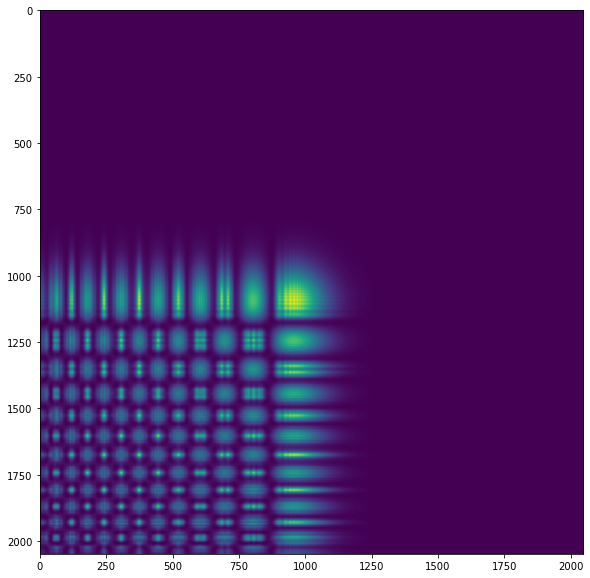
Initial Intensity:
I have attempted to write Fresnel diffraction manually before trying out LightPipes, but I had problems where I had weird edge intensities that do not exist. However, I did not get my intensity cut up like shown above. Additionally, papers I've read have results showing that Airy beams would shift diagonally during propagation in spatial domain, but it doesn't seem like it is the case here. If anyone has any insight on that part, that would be great, however it might also just be me not properly understanding the theory.