 github-actions[bot]
commented
3 years ago
github-actions[bot]
commented
3 years ago Object Detection and Tracking in 2020 by Borijan Georgievski
Object Detection and Tracking in 2020
[ ](https://medium.com/@ Borijan.Georgievski?source=post_page-----f10fb6ff9af3--------------------------------)
[Borijan Georgievski](https://medium.com/@ Borijan.Georgievski?source=post_page-----f10fb6ff9af3--------------------------------)
Apr 14, 2020 · 15 min read

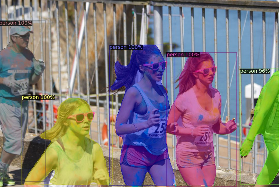
Mask R-CNN output on this image
Choosing an object detection and tracking approach for an application nowadays might become overwhelming. This article is an endeavor to summarize the best methods and trends in these essential topics in computer vision.
Nowadays, the problem of classifying objects in an image is more or less solved, thanks to huge advances in computer vision and deep learning in general. The publicly available models trained on large amounts of data further simplifies this task. Accordingly, the computer vision researching community has shifted focus in other very interesting and challenging topics, such as adversarial image generation, neural style transfer, visual storytelling, and of course, object detection, segmentation and tracking.
We shall start off by paying homage to the long-established methods, and afterwards explore the current state-of-the-art.
The Old School
Object detection has been around for quite a while; the traditional computer vision methods for object detection appeared in the late 90s. These approaches utilize classic feature detection, combined with a machine learning algorithm like KNN or SVM for classification, or with a description matcher like FLANN for object detection.
The most notable feature detection algorithms are arguably SIFT and SURF as feature descriptors, and FAST for corner detection. The feature descriptors use a series of mathematical approximations to learn a representation of the image that is scale-invariant. Some of these old school methods could sometimes get the job done, but there is a lot more we can do.

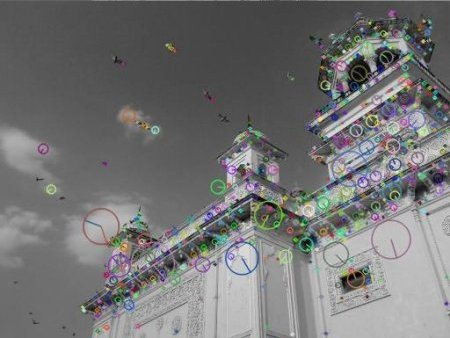
SIFT feature keypoints from OpenCV
As for object tracking, it seems like the traditional methods stood the test of time better than the object detection ones. Ideas like Kalman filtering, sparse and dense optical flow are still in widespread use. Kalman filtering entered hall of fame when it was used in the Apollo PGNCS to produce an optimal position estimate for the spacecraft, based on past position measurements and new data. Its influence can be still seen today in many algorithms, such as the Simple Online and Realtime Tracking (SORT), which uses a combination of the Hungarian algorithm and Kalman filter to achieve decent object tracking.
The Novel Advancements of Object Detection
R-CNN
Back in 2014, Regions with CNN features (R-CNN) was a breath of fresh air for object detection and semantic segmentation, as the previous state-of-the-art methods were considered to be the same old algorithms like SIFT, only packed into complex ensembles, demanding a lot of computation power and mostly relying on low-level features, such as edges, gradients and corners.
The R-CNN system is comprised of three main modules. The foremost module extracts around 2000 region proposals using a segmentation algorithm called selective search, to figure out which parts of an image are most probable to contain an object. Selective Search applies a variety of different strategies, so it can handle as many image conditions as possible. The algorithm scans the image with windows of various scales, and looks for adjacent pixels that share colors and textures, while also taking lightning conditions into an account.
The second module is a large convolutional neural network that extracts a fixed-length feature vector from each proposal that is returned from the selective search. Regardless of the size or aspect ratio, the candidate region undergoes image warping to have the required input size. Lastly, the final module classifies each region with category-specific linear SVMs.

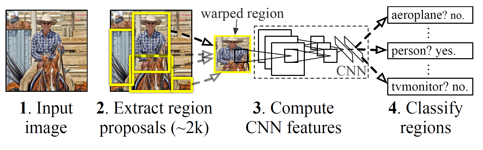
R-CNN framework
R-CNN is very slow to train and test, and not very accurate by today’s standards. Nevertheless, it is an essential method that paved the way for Fast R-CNN, and the current state-of-the-art Faster R-CNN and Mask R-CNN.
Fast R-CNN
Fast R-CNN was proposed by one of the authors of R-CNN, as a worthy successor. One big improvement over R-CNN is that instead of making ~2000 forward passes for each region proposal, Fast R-CNN computes a convolutional feature map for the entire input image in a single forward pass of the network, making it much faster. Another improvement is that the architecture is trained end-to-end with a multi-task loss, resulting in simpler training.
The input for Fast R-CNN is an image, along with a set of object proposals. First, they are passed through a fully convolutional network to obtain the convolutional feature map. Next, for each object proposal, a fixed-length feature vector is extracted from the feature map using a region of interest (RoI) pooling layer. Fast R-CNN maps each of these RoIs into a feature vector using fully connected layers, to finally output softmax probability and the bounding box, which are the class and position of the object, respectively.

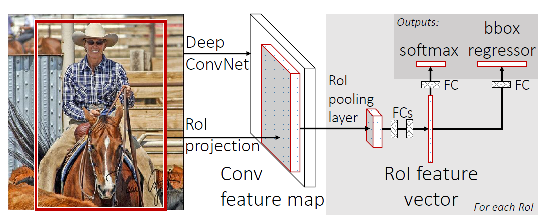
Fast R-CNN framework
Faster R-CNN
It turns out that Fast R-CNN is still pretty slow, and that is mostly because the CNN is bottlenecked by the aforementioned region proposal algorithm, selective search. Faster R-CNN solves this by abandoning the traditional region proposal method, and relying on a fully deep learning approach. It consists of two modules: a CNN called Region Proposal Network (RPN), and the Fast R-CNN detector. The two modules are merged into a single network and trained end-to-end.
The authors of Faster R-CNN drew inspiration from the attention mechanism when they designed RPN to emphasize what is important in the input image. Creating region proposals is done by sliding a small network over the last shared convolution layer of the network. The small network requires a (n x n) window of the convolutional feature map as an input. Each sliding window is mapped to a lower-dimensional feature, so just like before, it is fed to two fully connected layers: a box-classification and box-regression layer.
It is important to mention that the bounding boxes are parametrized relative to hand-picked reference boxes called anchors. In other words, the RPN predicts the four correction coordinates to move and resize an anchor to the right position, instead of the coordinates on the image. Faster R-CNN is using 3 scales and 3 aspect ratios by default, resulting in 9 anchors at each sliding window.

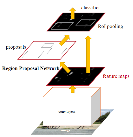
Faster R-CNN framework
Faster R-CNN is considered state-of-the-art, and it is certainly one of the best options for object detection. However, it does not provide segmentation on the detected objects, i.e. it is not capable of locating the exact pixels of the object, rather just the bounding box around it. In many cases this is not needed, but when it is, Mask R-CNN should be the first one to come to mind.
Mask R-CNN
The Mask R-CNN authors at Facebook AI Research (FAIR) extended Faster R-CNN to perform instance segmentation, along with the class and bounding box. Instance segmentation is a combination of object detection and semantic segmentation, which means that it performs both detection of all objects in an image, and segmentation of each instance while differentiating it from the rest of the instances.
The first stage (region proposal) of Mask R-CNN is identical to its predecessor, while in the second stage it outputs a binary mask for each RoI in parallel to the class and bounding box. This binary mask denotes whether the pixel is part of any object, without concern for the categories. The class for the pixels would be assigned simply by the bounding box that they reside in, which makes the model a lot easier to train.
Another difference in the second stage is that the RoI pooling layer (RoIPool) introduced in Fast R-CNN is replaced with RoIAlign. Performing instance segmentation with RoIPool results in many pixel-wise inaccuracies, i.e. misaligned feature map when compared to the original image. This occurs because RoIPool performs quantization of the regions of interest, which includes rounding the floating-point values to decimal values in the resulting feature map. On the other hand, the improved RoIAlign properly aligns the extracted features with the input, by avoiding any quantization altogether, rather using bilinear interpolation to compute the exact values of the input features.

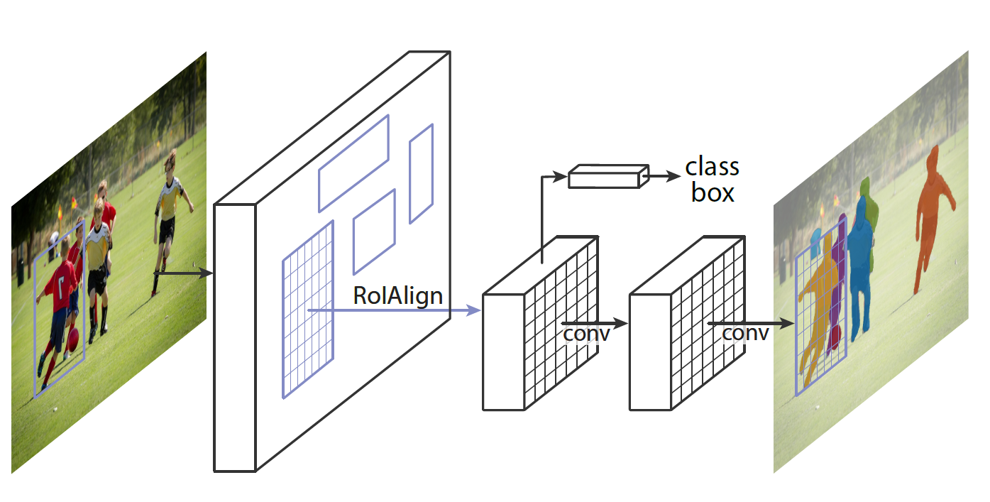
Mask R-CNN framework
YOLO
We are now switching focus from an accuracy-oriented solution, to a speed-oriented one. You Only Look Once (YOLO) is the most popular object detection method today, with a good reason. It is capable of processing real-time videos with minimal delay, all the while retaining respectable accuracy. And as the name suggests, it only needs one forward propagation to detect all objects in an image.
YOLO is designed in Darknet, an open source neural network framework written in C and CUDA, developed by the same author that created YOLO, Joseph Redmon. The last iteration is YOLOv3, which is bigger, more accurate on small objects, but slightly worse on larger objects when compared to the previous version. In YOLOv3, Darknet-53 (53-layer CNN with residual connections) is used, which is quite a leap from the previous Darknet-19 (19-layer CNN) for YOLOv2.
Unlike the previous YOLO versions that output the bounding box, confidence and class for the box, YOLOv3 predicts bounding boxes at 3 different scales on different depths of the network. The final object detections on the image are decided using non-max suppression (NMS), a simple method that removes bounding boxes which overlap with each other more than a predefined intersection-over-union (IoU) threshold. In such overlapping conflict, the bounding box with the largest confidence assigned by YOLO wins, while the others are discarded.

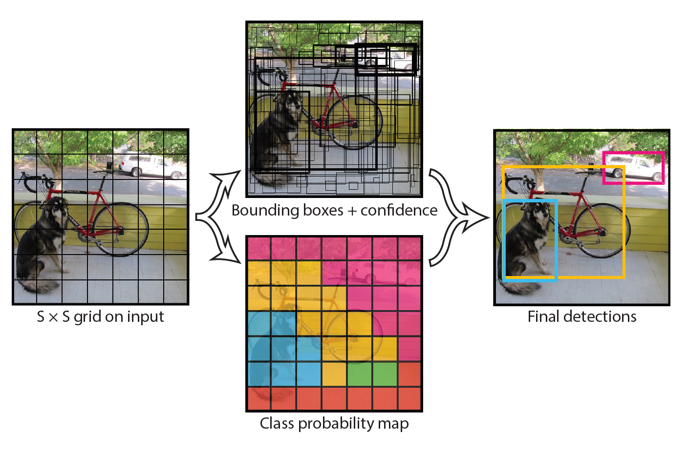
YOLO modeling object detection as a regression problem
Just like in Faster R-CNN, the box values are relative to reference anchors. However, instead of having the same handpicked anchors for any task, it uses k-means clustering on the training dataset to find the optimal anchors for the task. The default number of anchors for YOLOv3 is 9. It might also come as a surprise that softmax is not used for class prediction, but rather multiple independent logistic classifiers, trained with binary cross-entropy loss.
SSD
Single Shot MultiBox Detector (SSD) came out a couple of months after YOLO as a worthy alternative. Similarly to YOLO, the object detection is done in a single forward propagation of the network. This end-to-end CNN model passes the input image through a series of convolutional layers, generating candidate bounding boxes from different scales along the way.
As ground truth for training, SSD considers the labeled objects as positive examples, and any other bounding boxes that do not overlap with the positives are negative examples. It turns out that constructing the dataset this way makes it very imbalanced. For that reason, SSD applies a method called hard negative mining right after performing NMS. Hard negative mining is a method to pick only the negative examples with the highest confidence loss, so that the ratio between the positives and negatives is at most 1:3. This leads to faster optimization and a more stable training phase.

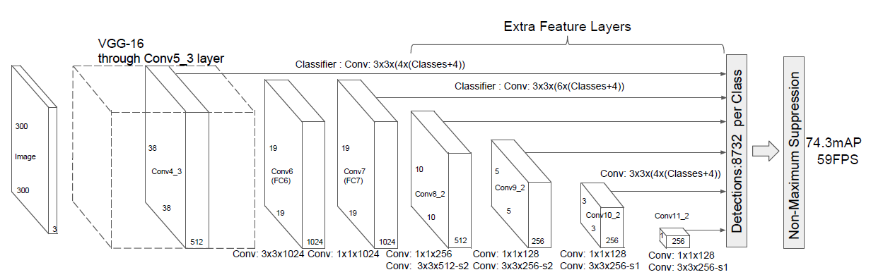
SSD architecture
In the image above that can be found in the official paper, we can see that the backbone network is VGG-16. However, nowadays we can often see SSD with a ResNet, Inception and even MobileNet backbone.
RetinaNet
RetinaNet was proposed back in 2017 by researchers from FAIR. It is also a one-stage framework like YOLO and SSD, which trades speed for worse accuracy than the two-stage frameworks like the R-CNN variations. The RetinaNet uses a ResNet + FPN backbone to generate a rich, multi-scale convolutional feature pyramid. As usual, two subnetworks are attached on top, one for classifying anchor boxes, and another one for generating offset from the anchor boxes to the ground-truth object boxes.

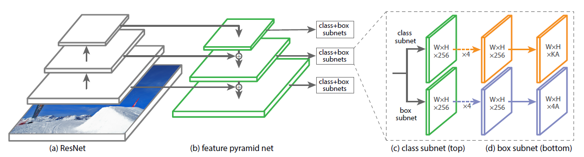
RetinaNet architecture
As mentioned before, imbalance of classes during training of dense detectors overwhelms the cross entropy loss. The innovative focal loss improves accuracy focusing training on a sparse set of hard examples, while limiting the number of easy negatives. This is done by reshaping the loss function to not value easy examples as much as the hard ones.

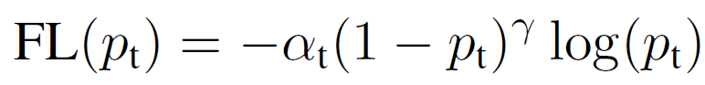
Focal loss definition, where α ∈ [0, 1] is a weighting factor addressing class imbalance, and γ is the focusing parameter
Introducing the weighting factor α is a common method for addressing class imbalance. The authors first experimented with α=0, but this yielded worse accuracy than the alpha-balanced form. You may also notice that when γ=0, the focal loss is equivalent to cross-entropy loss.
The Novel Advancements of Object Tracking
ROLO
For starters, we can check out Recurrent YOLO (ROLO), a single object tracking method that combines object detection and recurrent neural networks. ROLO is a combination of YOLO and LSTM. The object detection module uses YOLO to collect visual features, along with location inference priors. At each time-step (frame), the LSTM receives an input feature vector of length 4096, and returns the location of the tracked object.

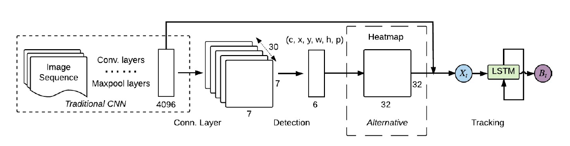
ROLO architecture
SiamMask
When it comes to single object tracking, SiamMask is an excellent choice. It is based on the charming siamese neural network, which rose in popularity with Google’s Facenet. Besides producing rotated bounding boxes at 55 frames per second, it also provides class-agnostic object segmentation masks. In order to achieve this, SiamMask needs to be initialized with a single bounding box so it can track the desired object. However, this also means that multiple object tracking (MOT) is not viable with SiamMask, and modifying the model to support that will leave us with a significantly slower object detector.
SiamMask demo with bounding box initialization
There are a couple of other notable object trackers that utilize siamese neural networks, such as DaSiamRPN, which won the VOT-18 challenge (PyTorch 0.3.1 code) and SiamDW (PyTorch 0.3.1 code).
Deep SORT
We have previously mentioned SORT as an algorithmic approach to object tracking. Deep SORT is improving SORT by replacing the associating metric with a novel cosine metric learning, a method for learning a feature space where the cosine similarity is effectively optimized through reparametrization of the softmax regime.
The track handling and Kalman filtering framework is almost identical to the original SORT, except the bounding boxes are computed using a pre-trained convolutional neural network, trained on a large-scale person re-identification dataset. This method is a great starting point for multiple object detection, as it is simple to implement, offers solid accuracy, but above all, runs in real-time.
TrackR-CNN
TrackR-CNN was introduced just as a baseline for the Multi Object Tracking and Segmentation (MOTS) challenge, but it turns out that it is actually effective. First off, the object detection module utilizes Mask R-CNN on top of a ResNet-101 backbone. The tracker is created by integrating 3D convolutions that are applied to the backbone features, incorporating temporal context of the video. As an alternative, convolutional LSTM is considered as well, but the latter method does not yield any gains compared with the baseline.
TrackR-CNN also extends Mask R-CNN by an association head, to be able to associate detections over time. This is a fully connected layer that receives region proposals and outputs an association vector for each proposal. The association head draws inspiration from siamese networks and the embedding vectors used in person re-identification. It is trained using a video sequence adaptation of batch hard triplet loss, which is a more efficient method than the original triplet loss. To produce the final result, the system must decide which detections should be reported. The matching between the previous frame detections and current proposals is done using the Hungarian algorithm, while only allowing pairs of detections with association vectors smaller than some threshold.
Tracktor++
The Multiple Object Tracking Benchmark makes it easier to find the most recent breakthroughs in MOT, thanks to its public leaderboard. The CVPR 2019 Tracking Challenge motivated progress in both accuracy and speed of the trackers. Tracktor++ dominated the leaderboard with a very simple, yet effective approach. This model predicts the position of an object in the next frame by calculating the bounding box regression, without needing to train or optimize on tracking data whatsoever. The object detector for Tracktor++ is the usual Faster R-CNN with 101-layer ResNet and FPN, trained on the MOT17Det pedestrian detection dataset.

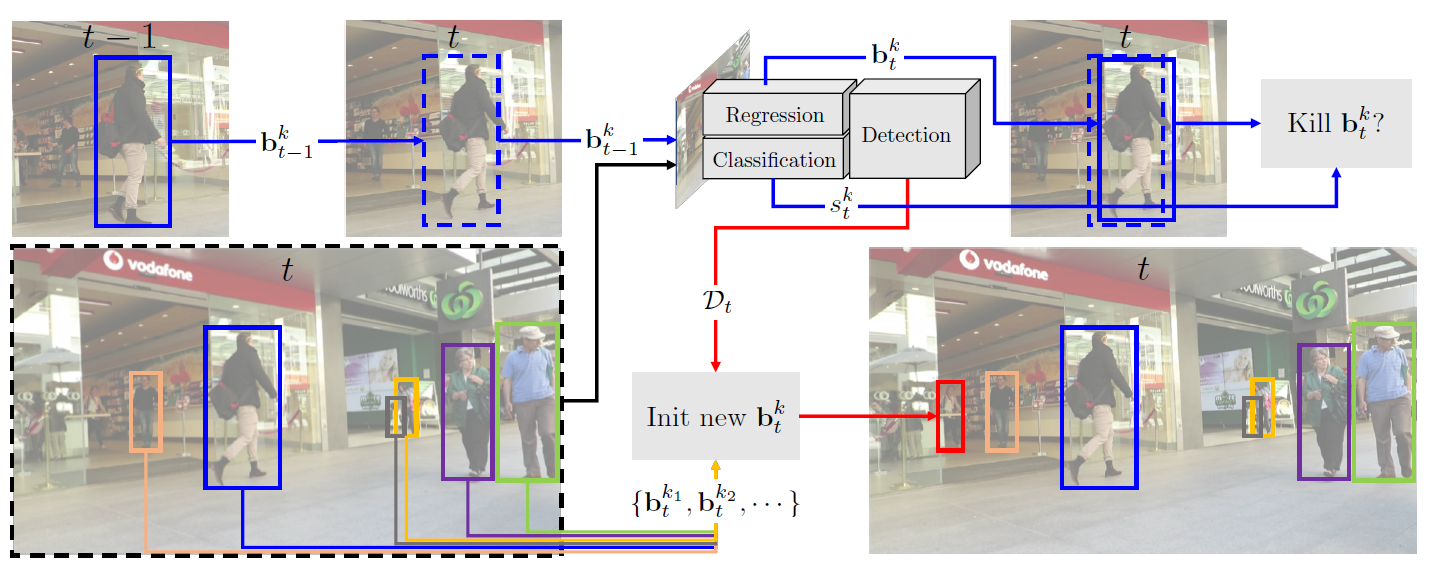
Tracktor++ framework
The main idea of Tracktor++ is to use the regression branch of Faster R-CNN for frame-to-frame tracking by extracting features from the current frame, and then using object locations from the previous frame as input for the RoI pooling process to regress their locations into the current frame. It also utilizes some motion models such as the camera motion compensation based on image registration, and short-term re-identification. The re-identification method caches deactivated tracks for a fixed number of frames, and then compares the newly detected tracks to them for possible re-identification. The distance between tracks is measured by a siamese neural network.
JDE
Joint Detection and Embedding (JDE) is a very recent proposal similar to RetinaNet that deviates from the two-stage paradigm. This single-shot detector is designed to solve a multi-task learning problem, i.e. anchor classification, bounding box regression and embedding learning. JDE uses Darknet-53 as the backbone to obtain feature maps of the input at three scales. Afterwards, the feature maps are fused together using up-sampling and residual connections. Finally, predictions heads are attached on top of the fused feature maps, which output a dense prediction map for the three tasks that were mentioned above.

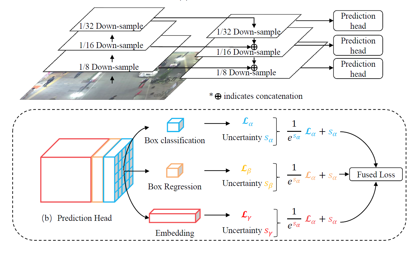
JDE architecture
To achieve object tracking, besides bounding boxes and classes, the JDE model also outputs appearance embedding vectors when processing the frames. These appearance embeddings are compared to embeddings of previously detected objects using an affinity matrix. Finally, the good old Hungarian algorithm and Kalman filter are used for smoothing out the trajectories and predicting the locations of previously detected objects in the current frame.
The Standoff
Now let us visualize and observe the performance of the four mentioned multiple object tracking methods. The following experiments are done on a machine running Ubuntu 18.04 with an Intel Core i7–8700 CPU and NVIDIA GeForce GTX 1070 Ti GPU. The sample videos are downloaded from the MOT17 test dataset. The resolution of all videos is 1920x1080, with various frames per second (FPS) and lengths, while the four chosen ones for this test are recorded at 30 FPS.
This test shows that there is no clear-cut winner, as it comes down to whether we want faster real-time inference, more accurate detections, or maybe additional segmentation. Additionally, it is established that the tracker performance is heavily dependent on the actual object detection module, so it is possible that we see an inferior tracker producing better results just because of its superior detector. With that being said, these are my thoughts:
- Deep SORT is the fastest of the bunch, thanks to its simplicity. It produced 16 FPS on average while still maintaining good accuracy, definitely making it a solid choice for multiple object detection.
- Tracktor++ is pretty accurate, but one big drawback is that it is not viable for real-time tracking. Our experiments yielded an average execution of 3 FPS. If real-time execution is not a concern, this is a great contender.
- TrackR-CNN is nice because it provides segmentation as a bonus. But as with Tracktor++, it is hard to utilize for real-time tracking, having an average execution of 1.6 FPS.
- JDE displayed decent performance of 12 FPS on average. It is important to note that the input size for the model is 1088x608, so accordingly, we should expect JDE to reach lower FPS if the model is trained on Full HD. Nevertheless, it has great accuracy and should be a good selection.
Code for Object Detection
Detectron2 is the second iteration of FAIR’s framework for object detection and segmentation. It includes a lot of pretrained models, which can be found at the models zoo. If you like PyTorch, I would suggest using Detectron2, it is basically plug-and-play!
If you prefer TensorFlow though, you can use the official TensorFlow Object Detection API, where you can find the code, along with the pretrained models zoo.
Faster R-CNN
- PyTorch: Detectron2
- TensorFlow: TF Object Detection API
- Tensorpack: link
Mask R-CNN
YOLO
- Original, in C: link
- C (for Windows): Windows users will need to use another repository for Darknet. This repo is an excellent alternative, but you will need to compile it yourself (it definitely lost me some time)
- PyTorch: link
SSD
- PyTorch: link
- TensorFlow: TF Object Detection API
RetinaNet
- PyTorch: Detectron2
- Keras: link
Code for Object Tracking
ROLO
- TensorFlow: link
SiamMask
- PyTorch 0.4.1: link
Deep SORT
TrackR-CNN
- TensorFlow 1.13.1: link
Tracktor++
- PyTorch 1.3.1: link
JDE
- PyTorch ≥ 1.2.0: link
That’s all folks, thank you for reading!
Choosing an object detection and tracking approach for an application nowadays might become overwhelming. This article is an endeavor to summarize the best methods and trends in these essential topics in computer vision.
Tags: deep_learning
via Pocket https://ift.tt/2Smvv9g original site
March 10, 2021 at 10:44AM