Add support to SeaExplorer gliders

cyrf0006 commented 8 years ago

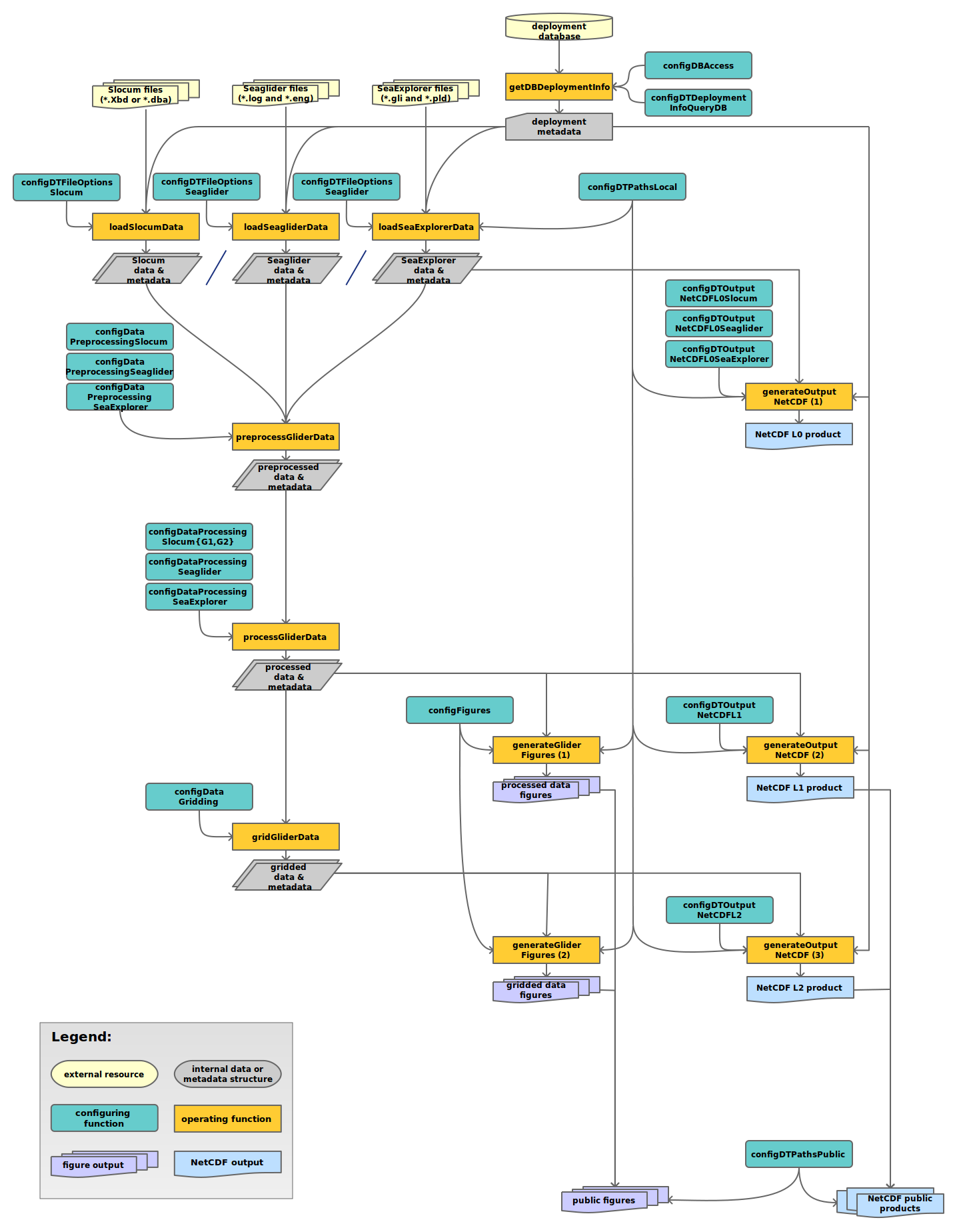
Attempt to include SeaExplorer gliders in the toolbox. Modifications to the toolbox would include functions such as:

loadSeaexplorerData.m
sx2mat.m
sxcat.m
sxmerge.m

Please refer any suggestion/questions to Frederic.cyr@mio.osupytheas.fr

cyrf0006 commented 8 years ago

Here are examples of navigations files (.gli.) and science files (.dat.), together with the glider's configuration (*.cfg) file that is read by the glider. For the moment, I need to manually edit this file to add extra fields during post-processing. These files should be read by an eventual loadSeaexplorerData.m function. This method is in development and may change in the future.

M78_example.zip

joanpau commented 8 years ago

Posting here some information from a mail discussion:

The format is a bit in between Slocum and SeaGlider I guess. There are 2 ascii files (CSV) per yo-. One for science ('dat') data and one for navigation data ('gli', that are sampled at a slower rate). I already read them and place them in a matlab struct with 2 different time vectors (see also the .mat file, troncated to reduce size). I think the only remaining step is to interpolate to a single time vector separate [DATA, META]. It should be easy.

cyrf0006 commented 8 years ago

I have written an early version of a function such as [meta, data] = loadSeaexplorerData(...) that is in the style of what is found in the toolbox for Slocum and SeaGlider. See attached the output this function, respecting the toolbox convention (variables names are different though...). I am not ready to share the code now, I would like to check first how it behaves with the rest of the toolbox.

Is there an easy way to check how the toolbox can read these data and do the full processing (Quality control, thermal lag correction, export to netCDF, etc.)? Maybe a real example of a script 'main_glider_data_processing_dt.m' that is used for another glider would be helpful at this stage? Also, would it be helpful to 'translate' variables names or the toolbox should be able to process any new variable?

For info, SeaExplorer saves much less variables than Slocum or SeaGlider. In the file attached, only 43 variables are present, including science and navigation parameters. This glider also include a new type of FDOM measurement (Tryptophan, Phenantrene, Naphtalene and other hydrocarbons).

Thanks for any feedback.

sxExample.mat.zip

joanpau commented 8 years ago

Although there are two main scripts, one for real time and one for delayed time processing, they are almost identical and we can focus on the delayed time one: main_glider_data_processing_dt. This script is used to process the data (for all glider types) on a per deployment basis. The glider type is specified in the deployment metadata, and the data loading and processing options are loaded from the configuration functions. You can take a look to the outline, and read the details in the help page and the code itself.

In the original code, deployment metadata is queried from a database with getDeploymentInfoDB. You can modify the main script to call your own function getDeploymentInfoLocal (or whatever you want to call it) to supply the metadata of the deployments to process. The output requirements are explained in the help comment:

The returned struct DATA should have the following fields to be considered 
a deployment structure:
  DEPLOYMENT_ID: deployment identifier (invariant over time).
  DEPLOYMENT_NAME: deployment name (may eventually change).
  DEPLOYMENT_START: deployment start date (see note on time format).
  DEPLOYMENT_END: deployment end date (see note on time format).
  GLIDER_NAME: glider platform name (present in Slocum file names).
  GLIDER_SERIAL: glider serial code (present in Seaglider file names).
  GLIDER_MODEL: glider model name (like Slocum G1, Slocum G2, Seaglider).
The returned structure may include other fields, which are considered to be
global deployment attributes by functions generating final products like
GENERATEOUTPUTNETCDF.

Notes:
  Time columns selected in the query should be returned as UTC timestamp
  strings in ISO 8601 format ('yyyy-mm-dd HH:MM:SS') or other format accepted
  by DATENUM, and are converted to serial date number format. 
  Null entries are set to invalid (NaN).

You could return SeaExplorer in the model field. Also be aware that, according to the time note, you should provide the start and end fields as a serial date number representing the corresponding date in UTC (not local time). Here there is a real example from our configuration:

deployment =

                   deployment_id: 159
                 deployment_name: 'JERICO_TNA_Sardegna_Jan2013_sdeep03'
                deployment_start: 7.3527e+05
                  deployment_end: 7.3531e+05
                     glider_name: 'sdeep03'
                   glider_serial: '541'
                    glider_model: 'SeaGlider 1KA'
          glider_instrument_name: 'SCB-SGDEEP003'
          glider_deployment_code: '0002'
                        abstract: [1x230 char]
                 acknowledgement: [1x123 char]
                          author: 'SOCIB Glider facility'
                    author_email: 'glider@socib.es'
                         creator: 'SOCIB Glider facility'
                   creator_email: 'glider@socib.es'
                     creator_url: 'http://www.socib.es/?seccion=observingFacilities&facility=glider'
                     data_center: 'SOCIB Data Center'
               data_center_email: 'data.centre@socib.es'
                     institution: [1x73 char]
          institution_references: 'http://www.socib.es/'
                      instrument: 'SCB-SGDEEP003'
         instrument_manufacturer: 'iRobot'
                instrument_model: 'SeaGlider 1KA'
                         license: 'Approved for public release. Distribution Unlimited.'
          principal_investigator: [1x113 char]
    principal_investigator_email: [1x113 char]
                         project: 'JERICO TNA'
                       publisher: 'SOCIB'
                 publisher_email: 'info@socib.es'
                   publisher_url: 'http://www.socib.es'
                         summary: [1x230 char]
                    calibrations: [1x1 struct]

The extra fields are used to populate the netcdf global attributes. You can set whatever fields you need in your institution. Also note the calibrations field, this can be used during the preprocessing to convert data from counts to engineering units.

Finally, you need to add a new case for the SeaExplorer glider type in the switch statements at lines 263, 398 and 443 of the main script.

You do not need to rename the raw variables. They are left unchanged in the L0 netCDF product, which you will need to describe in a configuration function configDTOutputNetCDFL0SeaExplorer. The variables are homogenized in the preprocessing configuration, configDataPreprocessingSeaExplorer. There you choose the raw variables that are used as time, latitude, longitude, temperature, etc. Unit conversion and factory calibration can be configured there too. Look at the help page of the data preprocessing function preprocessGliderData for reference.

Regarding the output you attached, you do not need to mimic the Slocum case in struct META. Actually, I would recommend to include only the metadata present in the raw files. According to the example files, this is just the the name of the source files and the column or variable names. So fields sources and sensors should be enough. And indeed, you do not need to call it that way, the term sensors is quite misleading here. It is called sensors for Slocum, and columns and PARAMS for Seagliders, because those are the terms used by the manufacturer in the format documentation and/or the glider manual. If the SeaExplorer documentation uses an specific term, take it. Otherwise, choose whatever you think is descriptive, variables or columns sound better to me. Probably you have already guessed that the information in the config field should be in the deployment metadata supplied by your function getDeploymentInfoLocal.

cyrf0006 commented 8 years ago

Ok that's perfect! I struggled to add these meta info (glider ID, deployment name, etc.) earlier in the process by modifying the configuration file. Much wiser how you suggest, e.g., by creating getDeploymentInfoLocal.

Another question of interest for anyone who would process such data: For some reasons, there might be errors in Lat/Lon/Time in the raw data (for example if the computer reset during deployment). These errors (only few bad points) will appear in netCDF_L0. Should I leave them anyway or correct them prior to save the netCDF_L0?

joanpau commented 8 years ago

The L0 output product contains exactly the same information than the raw data files, just gathering all the data from the whole deployment in the same file instead of having it spread over several hundred files.

If some points are to be discarded, this can be done in the preprocessing or processing. Actually, this is already done for the Slocum case, where the gps fixes are checked against the gps status variable. How to do it for the case of the SeaExplorer depends on how this errors are reflected in the raw data. I can not guess how a computer restart might create wrong timestamps or bad position readings. How do that bad points look like?

cyrf0006 commented 8 years ago

How do that bad points look like?

latitude = 0.0 longitude = 0.0

Thanks for the reply. I will write a new function that does the check during preProcessing and correct if necessary.

joanpau commented 8 years ago

That is really bad, because this is in fact a valid position reading... If those (0.0, 0.0) coordinates mean an uninitialized position measurement, SeaExplorer developers should consider to use NaN or some invalid value instead. (Something similar happens with the CTD in Slocums: all-zero readings in the initial lines of some files).

Anyway, the proper stage to detect those bad points would be in a quality control check, somewhere between preprocessing and processing. A simple domain test, configured according to the expected coverage of the deployment, would flag them as invalid. Please note that there is no such qc stage in the current version, although it is under development.

As a workaround, you can discard them in a custom made conversion function, and set it in the preprocessing configuration in your configDataPreprocessingSeaExplorer. nmea2deg is the conversion used for Slocums and Seagliders.

cyrf0006 commented 8 years ago

Other random but hopefully relevant comments/questions.

Are you generally working with Octave or Matlab? I guess Octave because a 'if' statement in posixtime.m was not implemented for Matlab. I fixed it.
This raises another remark. In the function findThermalLagParams.m you use fmincon.m which is part of the Matlab optimization toolbox. Have you ever tried a workaround for those you don't have this toolbox? Such as using fminsearch.m maybe?
Seaexplorer constructor have changed variables names from earlier glider generations. For the moment I was renaming before saving netCDF_L0. Is it a wrong idea (considering what you said in an earlier post about L0)?
what does the configDataProcessingSeaexplorer.m look like if a pumped CTD is used? (e.g. do we need to compute flow speed?)
In my case, processGlider.m is applied on data with both spikes and with NaNs (i.e. empty values still not filled). This causes problems for example when computing salinity from the CTD (sw_salt.m). Shouldn't NaNs and spikes be removed before?

joanpau commented 8 years ago

The toolbox is meant to be compatible with both MATLAB and (recent versions of) Octave.
The use of fmincon from the Optimization Toolbox in the (optional) thermal lag parameter estimation is the only point where we miss a replacement in Octave. A compatible package will be great, maybe a wrapper around nlopt or some other optimization library. I did not tried fminsearch (note it is for unconstrained optimization).
Yes, do not rename the variables when loading the data from the raw fils. The loading functions should just dump the data and metadata in the raw files to the interpreter, and from there to the L0 netCDF output with the least number of modifications. The preprocessing configuration allows setting a list of choices (in order of preference) for each set of sensors.
No, you do not need to compute the flow if the CTD is pumped. In fact, you may want to check whether the thermal lag correction is worth or not for your case. The correction might be marginal with pumped CTDs if the temperature gradients are not steep.
The processing functions in the toolbox accept NaNs in their input, and basically ignore them. The only problem will be if NaNs in the same sensor are not aligned (e.g. rows where all CTD measurements are NaN will not be a problem, but if there are rows with NaN in the temperature, and other rows with NaN in the conductivity, you will end up with NaN in the salinity in all those rows). For the spikes, they are again meat for the QC stage. I would ignore them right now, and focus on the integration. To inspect the data and design the QC test will be much more easier if the data is in netCDF format.

cyrf0006 commented 8 years ago

Thanks.

On this last point, however, it seems that the problem is more important. As an example, you can try to run
[data_processed, meta_processed] = processGliderData(data_preprocessed, meta_preprocessed, processing_options);

where the necessary input is attached here . The returned salinity is near zero. If I remove the NaNs and the spikes, the same call returns salinity in the good range.

joanpau commented 8 years ago

I inspected your example data, and I noticed the spikes in the conductivity. Of course, they cause spikes in the derived salinity, too. However, since the salinity derivation is time-local (earlier or later input values do not affect the current derived output value), they match the conductivity spikes perfectly. In your data, they sum up to the 0.25% of the whole data, the remaining 99.75% is ok:

load processGliderData_example.mat
[data, meta] = processGliderData(data_preprocessed, meta_preprocessed, processing_options);
plotTSDiagram('SData', data.salinity, 'TData', data.temperature);
sum(data.salinity < 37.75) / sum(~isnan(data.salinity))
bad_salt = data.salinity < 37.75;
plotTSDiagram('SData', data.salinity(~bad_salt), 'TData', data.temperature(~bad_salt));
figure;
plot(data.time, data.conductivity, '-b');
hold on;
plot(data.time(bad_salt), data.conductivity(bad_salt), '.r')

Also note how they are located always near the surface, and most of them at the beginning of the mission (zoom on that region):

figure
plot(data.time, data.depth, 'Color', [0.7, 0.7, 0.7])
hold on; axis ij;
plot(data.time(bad_salt), data.depth(bad_salt), '.r')

A sensor warm-up issue here maybe?

The above observation is of course false if you apply any non-trivial linear filter like the thermal lag correction to the conductivity signal. In that case, those wrong conductivity measurements will propagate to neighboring readings. You might circumvent this by using the filtered temperature with the raw conductivity as sources for the corrected salinity, so that the filtered conductivity is not used at all. This is what is done for G1 Slocums, although the reasons are different.

So this is clearly an issue to be addressed in the QC stage. Leave those spikes there by now to keep this issue separate from the integration, if you do not want to mess up your commit history. As a workaround you can remove those spikes in the conductivity during the preprocessing, setting your own conversion function.

cyrf0006 commented 8 years ago

Ok, my apologies! I was doing : plot(data.salinity)

But since some salinities are complex in the output, the result figure put salinities on the x-axis, which fooled me up. My mistake, sorry. Data are fine as you raised.

joanpau commented 8 years ago

Yes, the complex are introduced by those spikes in the conductivity. And I taking a closer look, it seems that the spikes are conductivity drops always at the end of an upcast, or at the beginning of the deployment. I wonder if the glider is at surface, and the CTD can not pump water through the conductivity cell...

cyrf0006 commented 8 years ago

Question: In the gridded data, there the dimension vector 'depth' and the gridded matrix 'pressure'. In SeaExplorer case, they are both calculated from the CTD_pressure. While the dimension depth is regular (1-m bins), the matrix pressure has slight variations from cast to cast. Why's that? And what is the best approach for further analysis (contour plot using depth or pressure?, for example)

joanpau commented 8 years ago

In the gridded data, glider trajectory data from the processing stage is converted into vertical instantaneous profiles defined at regular intervals of depth. Hence, each data variable is returned as a 2D grid, in addition of a vector of depth coordinates (vertical axis) and vectors of profile index, latitude, longitude, and time coordinates (horizontal axis). From the documentation:

%    Each cast identified in DATA_PROC is converted to an instantaneous 
%    vertical profile. The position and time coordinates of the new profile are
%    the mean values of the respective coordinates in the cast. All profiles 
%    are defined at the same depth coordinates, computed as the depth range of
%    the whole trajectory divided into regular intervals of given resolution. 
%    The cast data is interpolated over the new depth grid binning the readings 
%    that lay in the corresponding depth intervals.

Here we look the pressure as a measurement variable similar to temperature or salinity, and hence is also presented in the gridded data. The depth, however, is regarded as a coordinate reference variable, the same as time, latitude and longitude, providing the location of the measurements in space-time.

Of course this is just the default configuration, you can choose to not include the pressure in the list of gridded variables, or to use it as the vertical coordinate reference variable, or both.

socib / glider_toolbox

Add support to SeaExplorer gliders #2