FrieseWoudloper commented 4 years ago

It would be great when methods for making models and predictions better explainable would be made available through tidymodels and could be added to a workflow, for example like the ones in the DALEX and iml package. Are there any plans to do this?

topepo commented 4 years ago

Those packages would just need to make some changes to the code that makes predictions. I suspect that DALEX is nearly there since it works with parsnip and that should be the same as what a workflow would need. @pbiecek

I don't think that we would make any packages in this area since the existing ones cover all of the ground.

The best thing that you can do is to put in DALEX and iml GH issues with reproducible examples using a workflow.

pbiecek commented 4 years ago

Thanks, We are working on effortless integration of DALEX with tidymodels (Now it is also possible, but requires the manual preparation of a suitable predict function. It is difficult to do this automatically without knowing the internal structure of objects).

The plan is to prepare a tutorial on how to use these packages together, something like this chapter for DALEX+mlr3 https://mlr3book.mlr-org.com/interpretability-dalex.html.

@topepo It would be fantastic to have for tidymodels a documentation of the object interfaces. For example, for farimodels, we have something like this UML class diagram, which makes it very easy to integrate this tool with others.

https://github.com/ModelOriented/fairmodels/blob/master/man/figures/class_diagram.png

topepo commented 4 years ago

Is there a tool that generates the diagram from a codebase (or other source)? I don't know that we will generate this by hand.

That's said, I can give you any details that you need regarding interfaces.

topepo commented 4 years ago

Also, we would be very happy to include a DALEX and ModelOriented tutorial on tidymodels.org

pbiecek commented 4 years ago

Sounds great! I'd need to extract (if possible) following information out of the trained model:

A. the task that is being performed (classification, regression, something else), B. interface to the predict function, which will return numeric scores (probabilities for classification, predictions for regression, and so on) C. data that was used for training for the model, in a format that can be used by the prediction function from point B. D. unique name/identifier of the model (if there is such a thing, we try to put unique model identifiers on the charts so that it is easier to remember which model is presented, but we can also generate a new name).

As far as data is concerned, I understand that there are at least two stages: raw and after processing with recipes. In the case of points B and C, I need to extract data from the model that the predict function will understand.

I'm guessing that the predict function understands data after processing with recipes. If the model does not contain the training data by itself, I would need some mechanism to provide the data in the form that the predict function understands. Maybe it is possible to draw from the model an object describing pre-processing steps from the receptions.

In the scikit learn, the pipeline contains both variable transformations and the model, so there the predict/predict_proba function can operate on raw data. The model itself does not contain data, so we supply them independently in the raw form. Pipeline's predict function understands how to work on raw data.

As far as UML diagrams are concerned, unfortunately, they are still made manually. We want to automate it somehow, but because S3 classes don't have strictly defined structures it's not easy.

topepo commented 4 years ago

Here's some technical details for your questions...

library(tidymodels)

## ── Attaching packages ────────────────────────────────────── tidymodels 0.1.1 ──

## ✔ broom     0.7.0      ✔ recipes   0.1.13
## ✔ dials     0.0.8      ✔ rsample   0.0.7 
## ✔ dplyr     1.0.0      ✔ tibble    3.0.3 
## ✔ ggplot2   3.3.2      ✔ tidyr     1.1.0 
## ✔ infer     0.5.2      ✔ tune      0.1.1 
## ✔ modeldata 0.0.2      ✔ workflows 0.1.2 
## ✔ parsnip   0.1.2      ✔ yardstick 0.0.7 
## ✔ purrr     0.3.4

## ── Conflicts ───────────────────────────────────────── tidymodels_conflicts() ──
## ✖ purrr::discard() masks scales::discard()
## ✖ dplyr::filter()  masks stats::filter()
## ✖ dplyr::lag()     masks stats::lag()
## ✖ recipes::step()  masks stats::step()

What is the task being performed?

Our models contain a mode attribute that describes the type of problem. Currently, the modes are "unknown", "classification", and "regression". More modes will follow when we start integrating survival analysis models.

Before being assigned, the mode for a model specification is "unknown". A specification cannot be fit without an unknown mode.

Here's an example:

knn_mod <- 
  nearest_neighbor(neighbors = 3) %>% 
  set_engine("kknn") %>% 
  set_mode("regression")

For parsnip, the $mode element gives you this:

knn_mod$mode

## [1] "regression"

For a workflow, you pull the model specification and get the mode:

knn_workflow <- 
  workflow() %>% 
  add_model(knn_mod) %>% 
  add_formula(mpg ~ .)

knn_workflow %>% 
  workflows::pull_workflow_spec() %>% 
  pluck("mode")

## [1] "regression"

Once the model is fit, the process is similar since the specification is a sub-element of the fit:

# parsnip: 

knn_mod %>% 
  fit(mpg ~ ., data = mtcars) %>% 
  pluck("spec") %>% 
  pluck("mode")

## [1] "regression"

# workflows:

knn_workflow %>% 
  fit(data = mtcars) %>% 
   workflows::pull_workflow_fit() %>% 
  pluck("spec") %>% 
  pluck("mode")

## [1] "regression"

Interface to the predict function

There is one consistent interface to the predict methods: predict(object, new_data, type). The possible types are listed here although the available types differ by model (as is true for base R).

The main rules that makes it different than base R predict functions are:

If n rows are in new_data, the predict method always produces a tibble with n rows.
Columns are named according to the type argument.
- For univariate, numeric point estimates, the column should be named .pred. For multivariate numeric predictions (excluding probabilities), the columns should be named .pred_{outcome name}.
- Class predictions should be factors with the same levels as the original outcome and named .pred_class.
- For class probability predictions, the columns should be named the same as the factor levels, e.g., .pred_{level}, and there should be as many columns as factor levels.
- If interval estimates are produced (e.g. prediction/confidence/credible), the column names should be .pred_lower and .pred_upper. If a standard error is produced, the column should be named .std_error. If intervals are produced for class probabilities, the levels should be included (e.g., .pred_lower_{level}).

Again, the prediction interface is the same for parsnip and workflow objects.

For example:

knn_mod %>% 
  fit(mpg ~ ., data = mtcars) %>% 
  predict(mtcars %>% head())

## # A tibble: 6 x 1
##   .pred
##   <dbl>
## 1  20.9
## 2  20.9
## 3  24.7
## 4  20.5
## 5  18.6
## 6  19.2

knn_workflow %>% 
  fit(data = mtcars)%>% 
  predict(mtcars %>% head())

## # A tibble: 6 x 1
##   .pred
##   <dbl>
## 1  20.9
## 2  20.9
## 3  24.7
## 4  20.5
## 5  18.6
## 6  19.2

A classification example with parsnip:

data("two_class_dat", package = "modeldata")
levels(two_class_dat$Class)

## [1] "Class1" "Class2"

glm_fit <- 
  logistic_reg() %>% 
  set_engine("stan") %>% 
  # Mode is automatically set for models with only one possible value
  fit(Class ~ ., data = two_class_dat)

predict(glm_fit, two_class_dat %>% head()) # 'class' is the default type

## # A tibble: 6 x 1
##   .pred_class
##   <fct>      
## 1 Class1     
## 2 Class1     
## 3 Class1     
## 4 Class1     
## 5 Class2     
## 6 Class2

predict(glm_fit, two_class_dat %>% head(), type = "prob")

## # A tibble: 6 x 2
##   .pred_Class1 .pred_Class2
##          <dbl>        <dbl>
## 1        0.513       0.487 
## 2        0.905       0.0947
## 3        0.646       0.354 
## 4        0.596       0.404 
## 5        0.433       0.567 
## 6        0.200       0.800

predict(glm_fit, two_class_dat %>% head(), type = "conf_int")

## # A tibble: 6 x 4
##   .pred_lower_Class1 .pred_upper_Class1 .pred_lower_Class2 .pred_upper_Class2
##                <dbl>              <dbl>              <dbl>              <dbl>
## 1              0.468              0.560             0.440               0.532
## 2              0.870              0.934             0.0656              0.130
## 3              0.598              0.691             0.309               0.402
## 4              0.496              0.694             0.306               0.504
## 5              0.368              0.503             0.497               0.632
## 6              0.148              0.264             0.736               0.852

predict(glm_fit, two_class_dat %>% head(), type = "pred_int")

## # A tibble: 6 x 4
##   .pred_lower_Class1 .pred_upper_Class1 .pred_lower_Class2 .pred_upper_Class2
##                <dbl>              <dbl>              <dbl>              <dbl>
## 1                  0                  1                  0                  1
## 2                  0                  1                  0                  1
## 3                  0                  1                  0                  1
## 4                  0                  1                  0                  1
## 5                  0                  1                  0                  1
## 6                  0                  1                  0                  1

Again, workflow objects have the same syntax.

This probably won't matter to your applications, but some model predictions can produce nested data frame columns. For example, if someone is doing quantile regression and wants 7 specific quantiles, the tibble produced by predict will have n rows and the .pred column would be a list of tibbles, each with 7 rows.

Data that were used for training for the model

We generally eschew saving the training set with the model objects (along with pre-computed things like residuals and fitted values). For large data sets, this is problematic and all of these values can be re-produced on demand. This is pretty consistent with the S language belief in laziness. The model object itself might save these, but that is model dependent.

One other reason is that, especially for recipes, the data used to fit the model are not the original data. If we do any pre-processing or feature engineering, we strongly suggest keeping that separate from the model object.

I'm guessing that the predict function understands data after processing with recipes. If the model does not contain the training data by itself, I would need some mechanism to provide the data in the form that the predict function understands. Maybe it is possible to draw from the model an object describing pre-processing steps from the receptions.

In the scikit learn, the pipeline contains both variable transformations and the model, so there the predict/predict_proba function can operate on raw data. The model itself does not contain data, so we supply them independently in the raw form. Pipeline's predict function understands how to work on raw data.

Yes, this. This separation of data manipulation and model fitting might impact you because someone would give you a parsnip object but has done other pre-processing that produced an intermediary data set that was given to the model. If you don't have a way to replicate this, giving the original data to the model function is a bad idea.

That's why most of our focus is on workflows; these bundle together the pre-process/feature engineering/data processing with the model.

For example, if we want to do PCA prior to the model:

pca_rec <- 
  recipe(Class ~ ., data = two_class_dat) %>% 
  step_normalize(all_predictors()) %>% 
  step_pca(all_predictors(), num_comp = 2)

glm_mod <- 
  glm_fit <- 
  logistic_reg() %>% 
  set_engine("stan")

glm_pca_wflow <-
  workflow() %>% 
  add_model(glm_mod) %>% 
  add_recipe(pca_rec)

# does the PCA and normalization steps before modeling:
glm_pca_fit <- 
  glm_pca_wflow %>% 
  fit(data = two_class_dat)
glm_pca_fit

## ══ Workflow [trained] ══════════════════════════════════════════════════════════
## Preprocessor: Recipe
## Model: logistic_reg()
## 
## ── Preprocessor ────────────────────────────────────────────────────────────────
## 2 Recipe Steps
## 
## ● step_normalize()
## ● step_pca()
## 
## ── Model ───────────────────────────────────────────────────────────────────────
## stan_glm
##  family:       binomial [logit]
##  formula:      ..y ~ .
##  observations: 791
##  predictors:   3
## ------
##             Median MAD_SD
## (Intercept) -0.4    0.1  
## PC1         -1.2    0.1  
## PC2          2.8    0.3  
## 
## ------
## * For help interpreting the printed output see ?print.stanreg
## * For info on the priors used see ?prior_summary.stanreg

Then predict() just needs the original data:

predict(glm_pca_fit, two_class_dat %>% head(), type = "prob")

## # A tibble: 6 x 2
##   .pred_Class1 .pred_Class2
##          <dbl>        <dbl>
## 1        0.514       0.486 
## 2        0.907       0.0928
## 3        0.646       0.354 
## 4        0.601       0.399 
## 5        0.436       0.564 
## 6        0.201       0.799

I know that you have a page on using parsnip models already, but standardizing on workflows is much easier. For many of api's use workflows behind the scenes (even if the user's argument values did not use them). If I were you, I would write S3 methods for workflows, then have other S3 methods that combine formula/model or recipe/model combinations to a workflow. That's what tune::tune_grid() and similar functions do.

Unique name/identifier of the model

We don't really have that.

pbiecek commented 4 years ago

Thank you. We'll take a closer look at these options

topepo commented 4 years ago

No problem. Let me know if you have more questions.

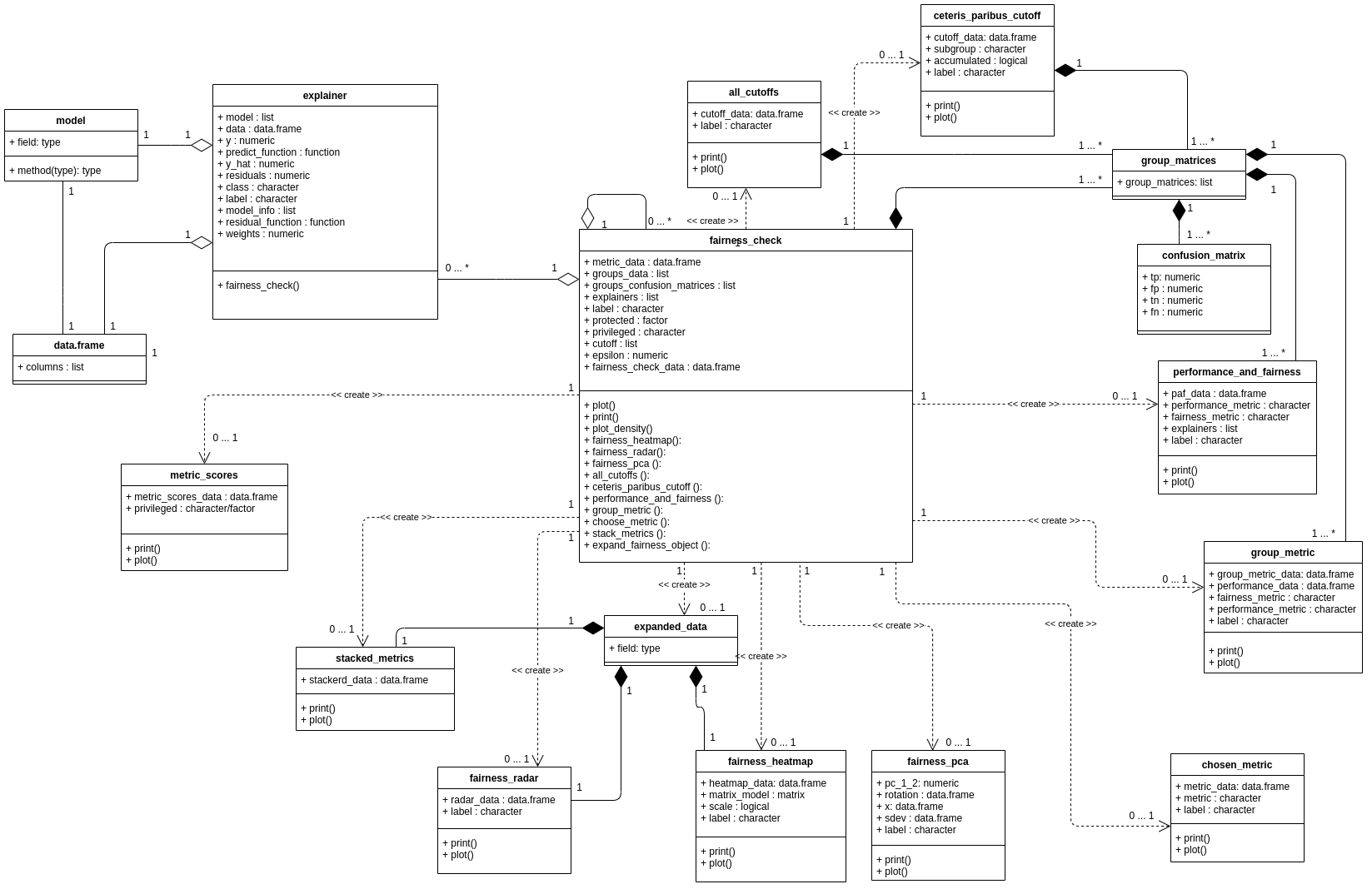
FrieseWoudloper commented 4 years ago

Thank you so much for your replies! Great to hear that there are plans to make it easier to integrate DALEX with tidymodels. @pbiecek: Can @Sponghop and I be of any assistance, for example with the tutorial? We are trying to learn tidymodels (rsample, recipes, parsnip, tune, workflows) and DALEX, and created a project using the Pima Indians Diabetes dataset and both packages. We're no tidymodels/DALEX experts, but willing to help.

pbiecek commented 4 years ago

@Sponghop sounds great, I'm going to prepare examples for classification model for DALEX::titanic

but it would be a great test if you could prepare a model with some advanced workflow for the Diabetes data. We would see if the solution for titanic can also be applied to the model you build

topepo commented 4 years ago

I made an example that uses recipes that could work as a template for a tidymodels.org article. So far, it looks like the same code that you used for parsnip can be used with a workflow.

In this example, the main predictor is a date column that gets engineered by a recipe into different features. Most everything in DALEX worked well (I think). However, using variable_effect() on the date seemed to trip it up. variable_attribution() appeared to do well but it converts the date to numeric in the plot.

Anyway, give it a look and let me know what you think.

Sponghop commented 4 years ago

@pbiecek this the link to the code we created for combining tidymodels with Dalex: https://github.com/Sponghop/dalex_tidymodels_example

We would be glad to hear your opinion about it and if we can be of further assistance.

maksymiuks commented 4 years ago

@Sponghop @topepo Thank You for those extensive examples! I've read through them and many things about how that integration should work are clear now. It looks doable to add tidymodels support without much interference in source code. I Will let You know once I finish branch with it and allow You to test it.

pbiecek commented 4 years ago

Thanks guys for all your examples.

@maksymiuks has prepared DALEXtra::explain_tidymodels function() which makes it easier to use DALEX for tidymodels.

Sponghop, examples with auto-tuned models are great. I still have to think whether it is possible to squeeze more in DALEX from data about the grid of tested models.

Here are some examples of DALEXtra::explain_tidymodels. We will prepare more descriptive vignette soon.

0. Prepare data

library("DALEX")
library("dplyr")
colnames(fifa)
fifa_small <- fifa %>%
  select(value_eur, age, 
         attacking_crossing:attacking_volleys, 
         defending_marking:defending_sliding_tackle)

1. Explanations operate on original feature space

Prepare recipes and train models. Here we reduce columns with step_pca and multiply columns with step_cut.

library("tidymodels")
library("recipes")
rec_pca <- recipe(value_eur ~ ., data = fifa_small) %>%
  step_cut(age, breaks = c(20, 25, 30)) %>%
  step_dummy(age) %>%
  step_pca(starts_with("attacking"), num_comp = 1, prefix = "attacking") %>%
  step_pca(starts_with("defending"), num_comp = 1, prefix = "defending") 

model <- boost_tree(trees = 100, tree_depth = 3) %>%
  set_engine("xgboost") %>%
  set_mode("regression")

wflow_pca <- workflow() %>%
  add_recipe(rec_pca) %>%
  add_model(model)  %>%
  fit(data = fifa_small)

Create an explainer

fifa_ex <- DALEXtra::explain_tidymodels(wflow_pca, 
                data = fifa_small[,-1], 
                y = fifa_small$value_eur,
                label = "Tidy-Boosting")

Try local and global explanations

model_performance(fifa_ex) %>% plot(geom = "histogram")
model_parts(fifa_ex) %>% plot()
model_profile(fifa_ex) %>% plot()
model_diagnostics(fifa_ex) %>% plot(variable = "y", yvariable = "y_hat")

lewandowski <- fifa_small["R. Lewandowski", ]

predict_parts(fifa_ex, lewandowski) %>% plot()
predict_profile(fifa_ex, lewandowski) %>% plot()
predict_diagnostics(fifa_ex, lewandowski) %>% plot()

2. Explanations operate on transformed feature space, after recipe

Prepare data (bake) and model

fifa_small_pca <- rec_pca %>% prep() %>% bake(fifa_small) %>% as.data.frame()

model_pca_raw <- workflow() %>%
  add_formula(value_eur ~ .) %>%
  add_model(model)  %>%
  fit(data = fifa_small_pca)

Create an explainer

fifa_ex_raw <- DALEXtra::explain_tidymodels(model_pca_raw, 
                          data = fifa_small_pca[,-1], 
                          y = fifa_small_pca$value_eur,
                          label = "Tidy-Boosting-Raw")

Try global and local explanations

model_performance(fifa_ex_raw) %>% plot(geom = "histogram")
model_parts(fifa_ex_raw) %>% plot()
model_profile(fifa_ex_raw) %>% plot()
model_diagnostics(fifa_ex_raw) %>% plot(variable = "y", yvariable = "y_hat")

lewandowski <- fifa_small_pca[21, ]

predict_parts(fifa_ex_raw, lewandowski) %>% plot()
predict_profile(fifa_ex_raw, lewandowski) %>% plot()
predict_diagnostics(fifa_ex_raw, lewandowski) %>% plot()

3. Explain two or model models in a single plot (Rashomon perspective)

Let's add Ranger model and explainer.

model_rf <- rand_forest(trees = 100) %>%
  set_engine("ranger") %>%
  set_mode("regression")

wflow_pca_rf <- workflow() %>%
  add_recipe(rec_pca) %>%
  add_model(model_rf)  %>%
  fit(data = fifa_small)

fifa_ex_rf <- DALEXtra::explain_tidymodels(wflow_pca_rf, 
                          data = fifa_small[,-1], 
                          y = fifa_small$value_eur,
                          label = "Tidy-Ranger")

And put both models in a plot.

plot(model_parts(fifa_ex), model_parts(fifa_ex_rf))
plot(model_profile(fifa_ex), model_profile(fifa_ex_rf))

tidymodels / planning

Add functionality to improve explainability to tidymodels #11

What is the task being performed?

Interface to the predict function

Data that were used for training for the model

Unique name/identifier of the model

0. Prepare data

1. Explanations operate on original feature space

2. Explanations operate on transformed feature space, after recipe

3. Explain two or model models in a single plot (Rashomon perspective)