IAU_Chrom 5.17+ Readme

Load chromatographic data from various sources like e.g. the Agilent Quadrupole‑MS or the Tofwerk TOFMS (sect. 2).
Have a look at your data with the viewing tools (viewers) on the plot windows of IAU_Chrom (sect. 3).
Define the species you want to analyse by loading the ms.info configuration file (sect. 2.5).
Integrate the signals of the defined substances and calculate the noise level on the respective baseline sections of the respective signals (sect. 4).
Save results in the form of an IDL binary file. That allows you to continue working on the experiment later on. Results can also be saved as text-files (sects. 2.2 and 4.1.3).
Specifically for mass spectrometric data, IAU_Chrom offers the possibility to analyse molecule fragment ratios if multiple ions are recorded per species. Use the fragment ratio calculation tool to do so (sect. 5).

Features

Technical Notes

Compatibility. IAU_Chrom is written in the IDL programming language on and for Windows machines (Win 7, 10). A version for Unix-based systems does not exist.
Version 5.02 and greater: Error handling is implemented which avoids total crashes for most errors. To avoid data loss in any case, save your experiment regularly.
To use IAU_Chrom on the system partition on your machine (C:\), it might be necessary to run IDL or the IDL virtual machine with elevated rights ("administrator mode").
To use the source code version (not pre-compiled), an IDL installation (v8.4 or higher) is required.

Start IAU_Chrom:

Runtime version, virtual machine only: run IAU_Chrom_vxxx.exe
Code version, IDL installed: open and run the IAU_Chrom\IAU_Chrom.pro from the root directory of the IAU_Chrom project.

The IAU_Chrom main widget is shown in Fig. 1.

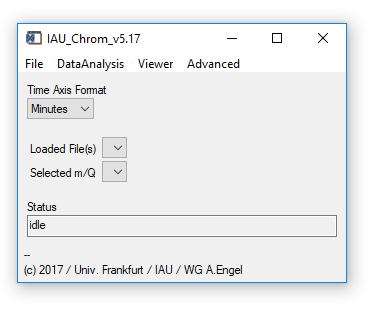
Fig. 1 - Main widget.

All further widgets (plots, tools) appear as soon as called/required.

Main widget: "File" tab

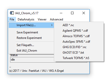
Fig. 2 - File menu on main widget.

'File' 'Import...': Import chromatographic (raw) data in different formats like netcdf (.nc/.cdf) or hdf5 (.h5) from different instruments. Choice is based on the instrument that produced the data.

To process measurement series, files should be named with an increasing index, like 01_name, 02_name or name_01 and so on. \"name" in this case is a constant string. A useful tool to rename and/or enumerate files is Ant Renamer, http://www.antp.be/software/renamer.
v5.13 and higher: IAU_Chrom also checks for a measurement timestamp in the data file; if loaded files are not sorted by ascending timestamp, it will ask you if you wish to sort by that quantity.

'File' 'Save Experiment': Saves the current set of loaded data, settings used for analysis and results together in one binary file *.sav. This file is only readable by IAU_Chrom (IDL proprietary format).

'File' 'Restore Experiment': Restores a *.sav / IDL binary file.

'File' 'Set Filepath...': Set the default directory where to look for save files etc.

'File' 'Exit IAU_Chrom': Closes the program.

(main widget) Time Axis Format: Change units of the x-axis to seconds or minutes. Chose the desired unit before loading data, otherwise results will be deleted. Restoring an experiment will automatically select the unit used in this experiment.

(main widget) Loaded Files / Selected m/Q: Dropdown-lists; appear as soon as data has been loaded or and experiment has been restored. Selecting one of the droplists will cause the plot window to appear and display the selection (Plot0).

Main widget: "DataAnalysis" tab

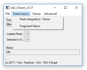
Fig. 3 - Main widget, data analysis tab.

'DataAnalysis' 'Peak Integration / Noise': Opens the integration widget. Requires: Chromatograms/experiment loaded, ms.info (see sect. 2.5).

'DataAnalysis' 'Fragment Ratios': Opens the fragment ratio calculator widget. See Ch. 5. Requires: Chromatograms/experiment loaded, ms.info (see sect. 2.5), fragments.info (see 2.7).

Main widget: "Viewer" tab

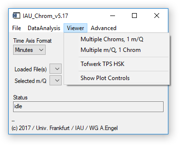
Fig. 4 - Main widget, viewer tab.

'Viewer' 'Multiple Chroms': Opens a viewer widget that can display an overlay of up to seven chromatograms (one specific m/q), see sect. 3. Uses plot window 0 (upper). Requires: Chromatograms/experiment loaded.

'Viewer' 'Multiple m/Q': Opens a viewer widget that can display an overlay of upt to seven m/q signals (one specific chromatogram), see sect. 3. Uses plot window 0 (upper). Requires: Chromatograms/experiment loaded.

'Viewer' 'TPS HSK': Opens a viewer widget for the housekeeping data recorded by the TPS module of the Frankfurt GC-TOFMS. Uses plot window 0 (upper). Requires: Chromatograms/experiment fromt the Tofwerk TOFMS loaded.

'Viewer' 'Show Controls': Opens a widget that allows you to control the plots' x- and y-ranges without using the „shiftkey-click-drag" method on the plot widgets. (Fig. 5).

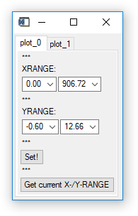
Fig. 5 - Plot controls widget.

Main widget: "Advanced" tab (scripting)

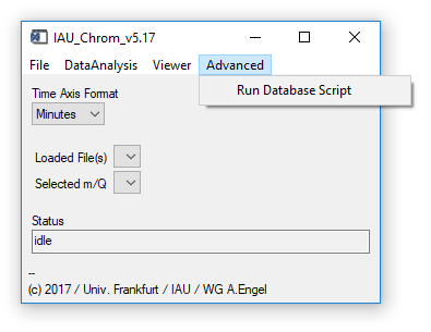
Fig. 6 - Main widget, advanced tab.

'Advanced' 'Run Database Script': Allows to run a script that defines experiments including e.g.

directory where data is found
path of an ms.info file
a definition which data should be imported (TOFMS, QPMS etc.)

The database script is a .csv table which contains a description of its use in the header, it is therefore not described in detail here.

Define your targets: "ms.info" config file

To analyse data, a configuration file is necessary that specifies target species' retention times and other parameters. It is named *ms.info by default. Before the ms.info file can be loaded, chromatograms have to be imported, see sect. 2.2.

A prompt to select an ms.info config file appears as soon as you call the integration widget from the DataAnalysis menu. It can also be re-loaded from the integration widget, see sect. 4. Be aware that if you integrate signals and then choose to re-load the ms.info config file, results will be reset (deleted) to ensure coherency of calculation results and configuration (integration parameters etc.).

The ms.info file can be opened and edited e.g. to add a new substance with a text editor like e.g. Notepad++. Make sure that the formatting stays intact after editing, i.e. leave no superfluous tabs, spaces, linefeeds etc.

Define molecule fragments and ratios: "fragments.txt" config file

Necessary to use the fragment ratios calculation tool, see sect. 5. Contains information on how which species fragments in 70 eV electron ionisation. E.g. CFC-12 (CF₂Cl₂) forms main ions of m/q 85 and 87, i.e. CF₂³⁵Cl⁺ and CF₂³⁷Cl⁺ with calculated m/q 84.96511 and 86.96216.

Data analysis: Tools to get an impression

Viewer: Multiple Chroms (MCV)

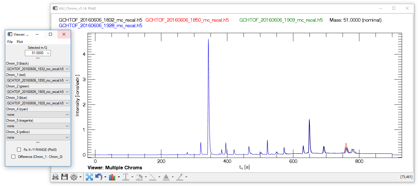
Fig. 7 - Multi Chrom Viewer widget with plot window.

The "multiple chroms viewer" (MCV) visualises a specific mass trace („Selected m/Q") in up to seven different chromatograms (Chrom_0 to Chrom_6). The checkbox "Difference Chrom_1-Chrom_0" calculates and displays the difference between the first and the second chromatogram (Chrom_1 is subtracted from Chrom_0).

MCV, file tab Exit. Closes the widget (plot stays opened).

MCV, plot tab Reset. Clears Plot0 (nothing displayed) and resets all selected values on the widget to default (nothing selected).

MCV, plot tab Recreate Textfields. Recreates the textfields on Plot0 at their correct positions.

Viewer: Multiple Masses (MMV)

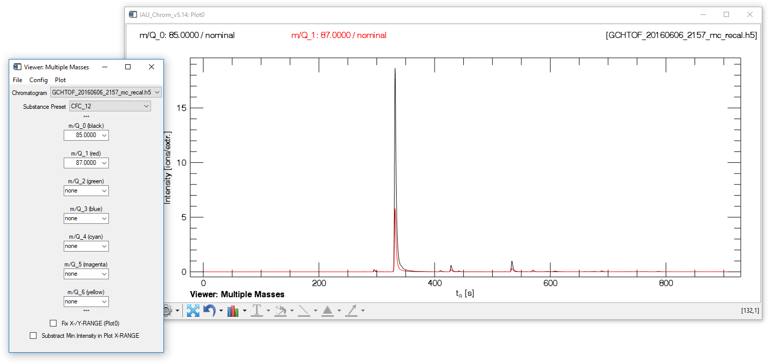
Fig. 8 - Mulit Mass Viewer widget with plot window.

The "multiple mass viewer" (MMV) can display up to seven different mass traces taken from one chromatogram (m/Q_0 to m/Q_6). Selecting a predefined set of mass traces belonging to one species in the ms.info config is possible after the ms.info has been loaded ("Substance Preset" droplist).

MMV, file tab Exit. Closes the widget (plot stays opened).

MMV, config tab (Re-)Load MSINFO. Allows the user to load an ms.info if none has been loaded or overwrite an already loaded ms.info.

MMV, plot tab Reset. Clears Plot0 (nothing displayed) and resets all selected values on the widget to default (nothing selected).

MMV, plot tab Recreate Textfields. Recreates the textfields on Plot0 at their correct positions.

MMV, plot tab Generate Legend. Displays a plot legend naming the selected mass traces.

Data Analysis: Integrate!

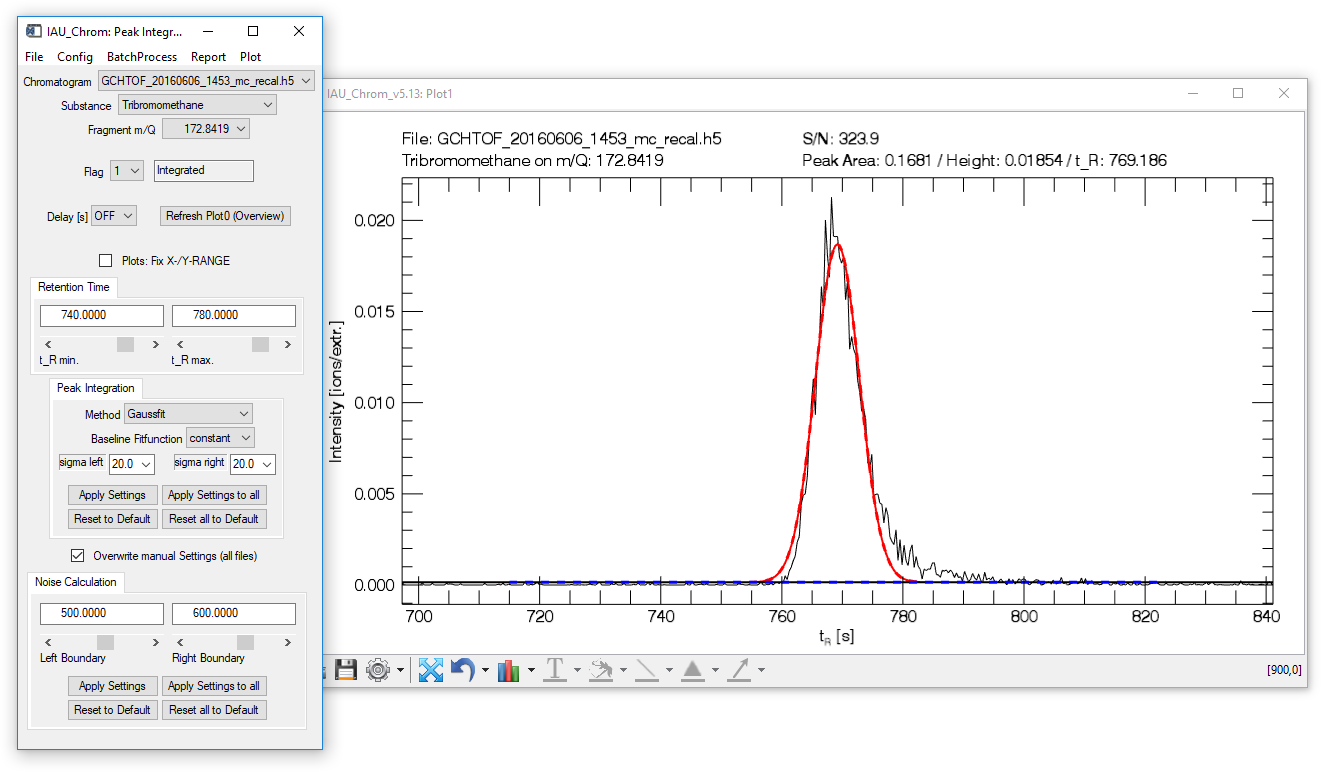
Fig. 9 - Peak integration widget with plot window. Integrated chromatographic signal shown.

data loaded
ms.info loaded
main widget data analysis peak integration/noise

The lower plot window (plot1, Fig. 9) shows the integrated chromatographic signal.

The upper plot window (plot0) shows the full mass trace of selected chromatogram and species. It can be refreshed by clicking the "Refresh Plot0 (Overview)" button on the integration widget.

Signal integration widget

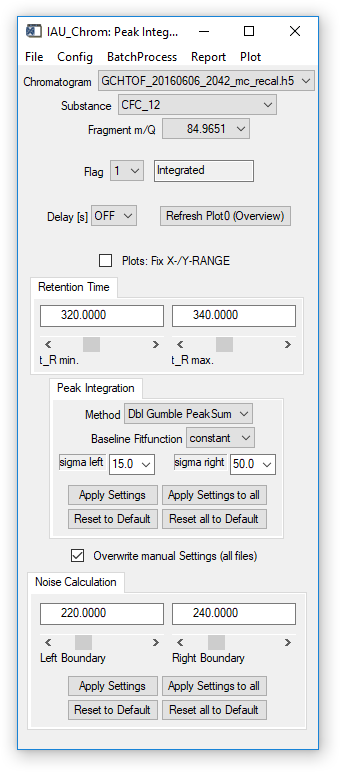
Fig. 10 - Integration widget.

Integration widget: "Config" tab

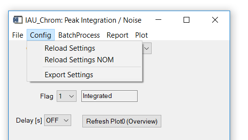
Fig. 11 - Integration widget, config tab.

'Config' 'Reload Settings': Reloads the ms.info file. Existing integration results will be deleted to avoid ambiguities.

'Config ' 'Reload Settings NOM': same as above exept that m/Q given as floating point numbers in the ms.info will be rounded to integers ('nominal m/Q').

'Config ' 'Export Settings': exports an ms.info file to a user-defined folder with the settings used in the selected chromatogram.

Integration widget: "BatchProcess" tab

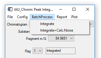
Fig. 12 - Integration widget, batch processing tab.

'BatchProcess' 'Integrate': All species defined in the ms.info will be integrated in all loaded chromatograms. During calculations, no results will be plotted.

'BatchProcess' 'Integrate+Calc. Noise': For all species defined in the ms.info, first the noise level will be calculated and then signals will be integrated (if present). Also here, no results will be plotted during calculations.

Integration widget: "Report" tab

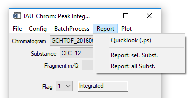
Fig. 13 - Integration widget, report tab.

'Report' 'Quicklook (.ps)': Generates a postscript file that contains diagnostic plots for all species that where integrated. The x-axis of each plot shows the measurement number, the y-axis show different parameters which are always normed to their mean value (e.g. peak area of a substance in a specific chromatogram divided by the mean peak area of this substance in all chromatograms).

'Report' 'Report: sel. Subst.': Generates a report-file (.txt) with integration results for the selected species in all chromatograms.

'Report' 'Report: all Subst.': Generates a report-files (.txt) with integration results for all species in all chromatograms.

Integration widget: "Plot" tab

‚Plot' ‚Recreate Textfields Plot1': Stellt die Textfelder auf Plot 1 an den korrekten Positionen wieder her.

'Report' 'Plot sel. Substance': Öffnet einen Diagnostik-Plot für die aktuell gewählte Substanz.

Signal integration: Settings

Flagging & Delay

The dropdown-menu "Flag" contains five different flags for selected chromatogram and substance. The following table lists the meanings of the flag values:

flag	meaning	explanation
-2	Bad Peak	To be set manually by the user. Denotes unusable / faulty data. If the integration is applied (to all chromatograms), this chromatogram will be skipped.
-1	No Peak Found	Automatically set. Indicates that the integration routine has found and integrated a signal in the selected data (chromatogram and m/Q).
0	Not Integrated	Initial state. Indicates that the integration was not (yet) called for this set of data. Initial state of all data when the integration widget is first started.
1	Integrated	Automatically set. Chromatographic signal found and integrated.
2	Integrated (man.)	Automatically set. Denotes integration settings that have been changed in comparison to other chromatograms (selected species).

Droplist "Delay": Lets you select a delay (pause) between integrations, i.e. if applying an integration setting to all chromatograms.

Checkbox "Overwrite manual Settings": Defines if manually edited integrations of individual chromatograms of the experiment are overwritten (checkbox set) or kept (box unchecked) if the function "apply settings to all" is called.

Retention time and peak integration

Note: See section 4.2.3 for further hints which settings to select under which circumstances.

t_R min. and t_R max.: selects the x-axis section / retention time section, within which a signal is expected (and should be integrated).

Peak Integration: Method. Selectes the integration method. Choices are Baseline, Gaussfit and different variants of a Gumble-Fit.

Peak Integration: Baseline Fitfunction. Different baseline functions are available, chose between constant (no inclination), linear (with inclination) und quadratic (2^nd order polynomial).

Peak Integration: Sigma left / Sigma right. These parameters determine, which data left and right of the signal apex are used to calculate the fit. 1 sigma is equivalent to the sigma (half width) of a Gaussian fit resembling the signal. The value you enter is a multiplier for this sigma value.

Integration: general tips

General goal here are precise and accurate results. A relative calibration scheme is assumed (multiple calibration measurements within the measurement series). The choice how to configure the signal fit relies on two basic, opposing conditions (within the measurement series you analyse):

1) Chromatography is very stable, the peak shape does not change a lot. 2) Peak shape changes.

In case 1), the Gaussian fit is a good choice in most cases. In this case, it is most important to "feed" as much data into the fit as possible. This will give you a very good (precise!) representation of the actual signal. For integration settings this means: use as high multiplier values (sigma left / sigma right) as possible. It does not matter if the shape of the signal is exactly matched by the fit, key here is representation, not resemblance. Accuracy is very good as long as the peak shape doesn't change significantly.

In case 2), it is better to chose integration settings so that the fit resembles the signal so that the changing signal shape is also present in the calculated fit. Otherwise, results might be inaccurate (although precision can still be good...).

Fig. 14 shows an example of an integrated signal. From the two signals found in the retention time section shown in the plot, the first signal is the target -- the first thing to do to configure the integration would be to set the retention time window so that only the fist signal lies within.

Note that the fit is composed of a solid and a dashed line, red for the peak and blue for the baseline. The solid line shows you, which data (x-coordinate) has been used for the fit. The dashed line shows the complete fit. The fit integration is always equivalent to ± 15 sigma.

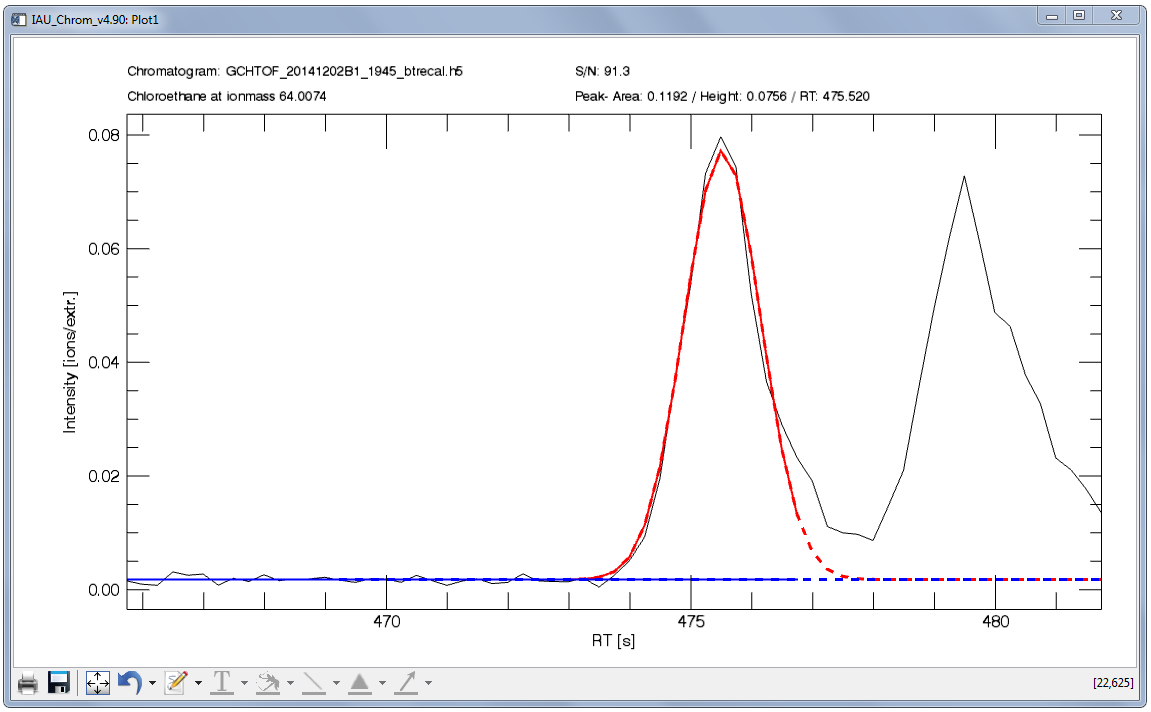
Fig. 14 - Integration plot. Black, solid line: m/Q intensity recorded over time (dI/dt). Red, solid line: data in this x-section are used to calculate the fit function. Red, dashed line: resulting fit curve. Blue: baseline.

To configure the sigma left / sigma right values in the example Fig. 14, a large value can be used for sigma left (e.g. 20) as there is no other signal to the left of the targeted peak. However to the right, there is another signal -- to get an accurate fit, no data points of the non-targeted signal may be used to calculate the fit. Consequently, a sigma right value of e.g. 2 has to be used.

Integration: methods

\'Baseline_dynamicRT\': (ms.info tag: \'bl\')

IAU_Chrom tries to detect a signal in the specified retention time window.
The peak detection algorithm returns peak parameters like estimated retention time or full width at half maximum (2 sigma).
Based on the sigma value from peak detection and the sigma multipliers on the integration widget, a retention time section "int_win" is determined where baseline fitting and peak integration will be performed.
At beginning and end of the int_win section, 6 data points on each side are used to calculate a baseline fit (order based on the selection on the integration widget).
All data points within int_win are then integrated after baseline subtraction.
although no actual peak fitting is performed, this method compensates for shifts in retention time as peak detection is used.

\'GaussFit\': (ms.info tag: \'gau\')

Peak detection and determination of int_win according to '\'Baseline_dynamicRT'.
Selection of data points to calculate the fit based on sigma multipliers (explanations see also sect. 4.2.3).
Calculation of the peak fit as a Gaussian distribution.
Integration of the fitted signal within ±15 sigma (you can't change this value).

\'Gauss_SGbase\': (ms.info tag: \'gau_SGbase\')

Based on \'GaussFit\'.
Peak detection and determination of int_win according to '\'Baseline_dynamicRT'.
In order to find a baseline, the data is smoothed with a Savitzky-Golay filter (nleft = nright = 3, sg_degree = 3). Finds the minima on the left and on the right side of the peak found with peak detection within the sigma left and sigma right interval using the smoothed data.
The so found baseline is applied to a gaussian fit by substracting it from the raw data and using NTERMS=3 for gaussfit.
Enforces a minimum number of datapoints per peak: 5 points within +- 2.5 sigma.
Integration of the fitted signal within ±15 sigma (you can't change this value).

\'GumbleFit\': (ms.info tag: \'gbl\')

Peak detection and determination of int_win according to '\'Baseline_dynamicRT'.
Selection of data points according to 'GaussFit'.
Calculation of the peak fit as a Gumble distribution.
Integration of the fitted signal within the sigma values you entered on the integration widget.

\'Dbl_Gumble_1stPeak\': (ms.info tag: \'dblgbl_1st\')

See 'GumbleFit'.
Assumes a double peak with the second (smaller) peak sitting on the right shoulder of the first (larger) peak.
'_1stPeak' the peak parameters of the first peak are returned by this function.

\'Dbl_Gumble_2ndPeak\': (ms.info tag: \'dblgbl_2nd\')

See 'GumbleFit' / 'Dbl_Gumble_1stPeak'
'_2ndPeak' the peak parameters of the second peak are returned by this function.

\'Dbl_Gumble_PeakSum\': (ms.info tag: \'dblgbl_sum\')

See 'GumbleFit' / 'Dbl_Gumble_1stPeak' / 'Dbl_Gumble_2ndPeak'
'PeakSum' the peak parameters of both peaks are returned (e.g. sum of areas peak 1 + peak 2) by this function.

\'Fix_2point_BL\': (ms.info tag: \'bl_fix\')

The first and last data point in the specified retention time window are used to calculate a line between these points (=baseline).
Integration of all data points in the retention time window after baseline subtraction.
If a noise level was calculated, results are only returned if the detected peak height is greater than the 1.5-fold noise level (otherwise, the result is 'no peak found').
If the integrated intensity (peak area) is below zero, a 'no peak found' is returned as well.
since this method does not use peak detection, it also doesn't compensate a shift in retention time during a measurement series. On the one hand side, this might reduce precision -- but on the other hand side, signals that are difficult to integrate with other methods might be feasible with this method due to its simplicity.

\'SavGol_BL\': (ms.info tag: \'SavGol_bl\')

Based on \'Baseline_dynamicRT\'.
In order to find a baseline, the data is smoothed with a Savitzky-Golay filter (nleft = nright = 3, sg_degree = 3). Peak detection and determination of int_win according to \'Baseline_dynamicRT\' - but using the smoothed data. Finds the minima on the left and on the right side of the peak found with peak detection within the sigma left and sigma right interval using the smoothed data.
In case of a constant baseline the lower minimum is used.
In case of a linear baseline the baseline is fitted through both minima.
Peak Area and Height are calculated by subtracting the baseline from the raw data.
Does not calculate Area, if at least one of sigma left and sigma right is lower than 3.

Noise calculation

To calculate a noise level on a specific m/Q, a retention time window (Left Boundary & Right Boundary, see Fig. 10) has to be defined. In this section of the x-axis, a 2^nd order polynomial fit is calculated. The noise level is then calculated as the 3-fold standard deviation of the differences (residuals) between fit and data points.

Data Analysis: Fragment Ratios

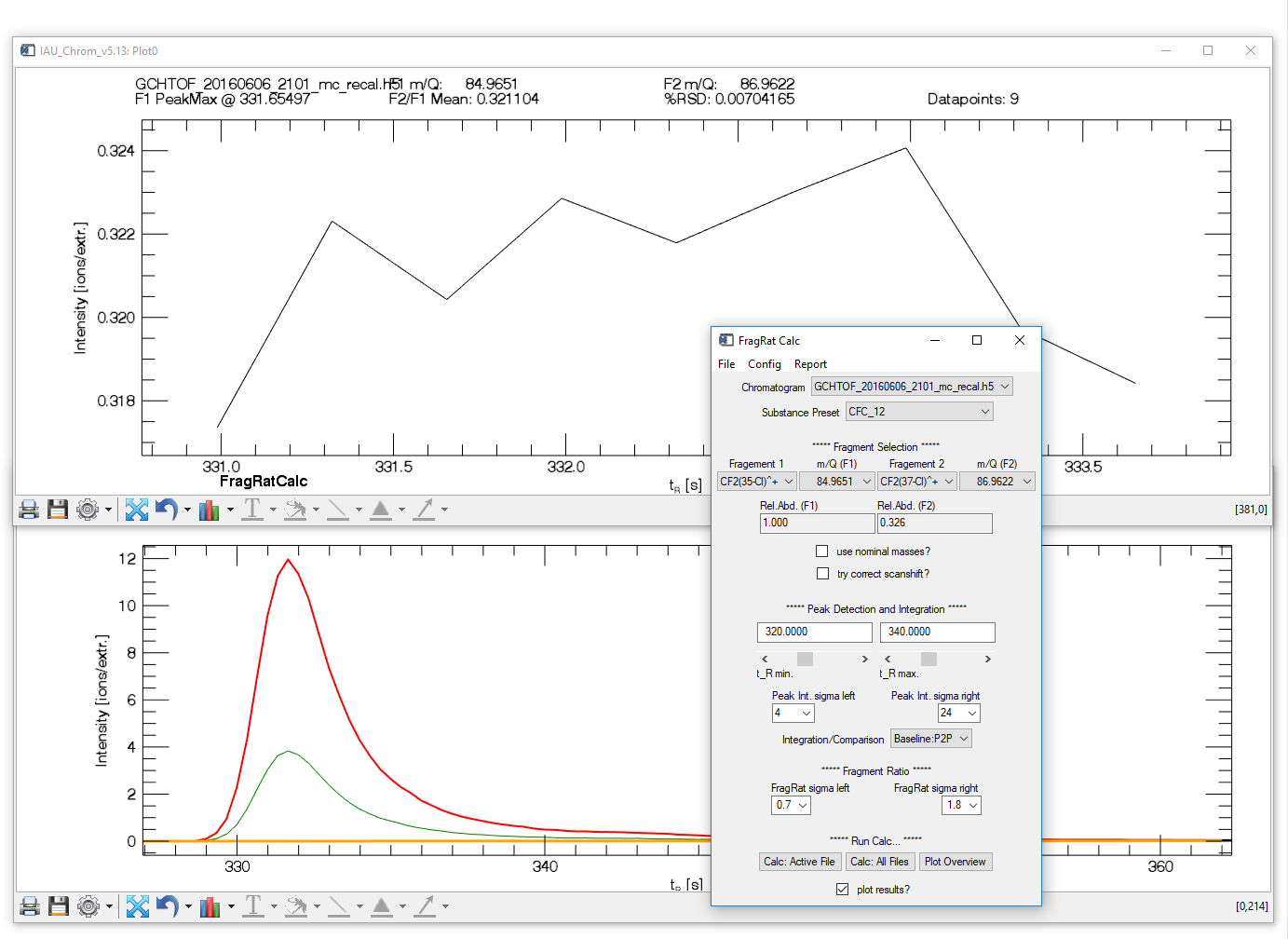
Fig. 15 -- Fragment ratio calculator widget with plots.

This tool can analyse ratios of different ions fragmented from a molecule. Prerequisite: chromatographic data and ms.info file loaded or experiment restored. Additionally requires: eifrags.txt - a config file that tells the software which signals to compare to analyse a specific substance. To match substance information from ms.info and eifrags.txt, substance names have to be spelled equally in both files (case-sensitive!).

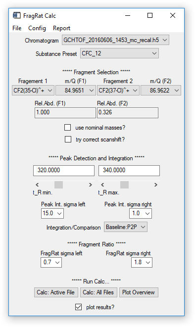
Fig. 16 - FragRat Calc widget.

Configuration options on the widget

Chromatogram, Substance Pre-set and Fragments: set as desired.
Use nominal masses: if checkbox is activated, ion masses (m/q) specified as decimal numbers will be rounded to integer values ("nominal masses"). If the data contains nominal and accurate m/q vectors, nominal values will be preferred. If data contains only accurate values, make sure to uncheck the box.
Try correct scanshift: if activated, a simple correction is applied to the result that compensates the temporal shift of intensity values of different m/q signals. Note that this is only a "data correction", not a correction of possible spectral skewing from the MS. Has no effect on TOFMS data.
t_R min, t_R max: retention time window; where the signal of interest is found in the chromatogram(s). Set the window so that an unambiguous identification of the signal is possible.
Peak int. sigma left/right: Required setting if peak fits should be used to derive the ratio, see next point (Comparison). The software will try to detect a signal (peak) in the specified retention time window. Sigma left and right specify the data (in multiples of ½ FWHM of a fit estimate returned by the peak detection algorithm) that is used to calculate a Gaussian fit of the detected signal. Change these values to get a fit that resembles peak and baseline.
Comparison: either select "Baseline/P2P" to perform a point-to-point comparison of data points or "Fit2Fit" to compare fitted curves to retrieve the ratio.
FragRat sigma left/right: Determines which data points are used to calculate the ratio. Numbers entered are multiples of sigma, i.e. ½ FWHM of a Gaussian peak representing the signal (see peak integration).

Some hints to get useful results

"save experiment" option (main widget): fragment ratio results and config file will not be saved. Make sure to save results as .txt (option on fragrat calc widget)
fragrat sigma left/right can strongly influence the result. Make sure to use equal values here if comparing different measurements.
Special note on scanning-type mass spectrometers, switching and recording m/q sequentially: ion composition in the ion source might have changed during the time it takes the instrument to switch from one m/q to another ("spectral skew"). A point-2-point ratio consequently might be biased ("comparing apples with apple-like pears"). To minimise the inaccuracy introduced by spectral skew, e.g. only points should be compared that are not located at the steepest parts of the signal flanks (max. dI/dt). The configuration options expressed in multiples of sigma can help in that respect, try e.g. sigma \< 1 in case of doubt.

What the report-file (.txt) tells you

File: data file name
m/q_f1: m/q of fragment 1
m/q_f2: m/q of fragment 2
ratio: mean ratio of all ratios calculated (point-2-point comparisons)
rsd: relative standard deviation of all ratios calculated
n_dp: number of data points used to calculate the mean ratio
RTp1: retention time at peak apex of fragment 1
dRT: temporal shift; retention time at peak apex of fragment 2 signal minus retention time at peak apex of fragment 1 signal
peakint_sl: sigma multiplier used for peak integration
peakint_sr: sigma multiplier used for peak integration
fragrat_sl: sigma multiplier used for determination of the retention time window within which to calculate the ratio
fragrat_sr: sigma multiplier used for determination of the retention time window within which to calculate the ratio
a_ratio: ratio of (fitted) peak areas
h_ratio: ratio of (fitted) peak heights

Amsoht / IDL_IAU_Chrom

readme