DVHToolkit

A GUI toolkit for visualizing and performing toxicity modelling and bootstrapping using Dose Volume Histogram files.

Extract information from Dose Volume Histogram files, calculate metrics such as D%, V% and fitting to NTCP models with methods of calculating the confidence intervals of the resulting parameters. By Helge Egil Seime Pettersen, Haukeland University Hospital, 2019.

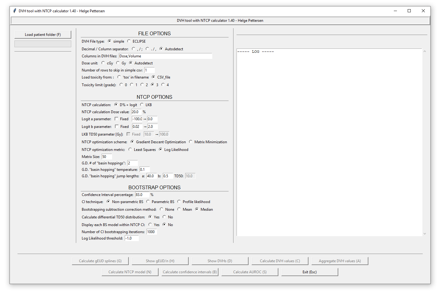
The program consists of a single window with some dialog options. Most of the buttons and options are documented with a tooltip, accessed by holding the pointer above the wanted option. All settings are saved upon exiting.

Current version: 1.67

FILE options

Before loading any patient / cohort folders containing CVS or ECLIPSE DVH files, the files to be opened has to be configured using the «FILE OPTIONS» part of the window. First, the file type has to be selected:

• CSV files: A simple CSV file is a DVH file that is either comma or semicolon separated, containing the columns «Dose» and «Volume». It is configured by choosing whether it is comma separated with period decimals (x.y, x.y), or semicolon separated with comma decimals (x,y; x,y): the autodetect option chooses semicolon if any are detected in the first line. Then, the columns has to be chosen. Use a comma-separated list without whitespace. The two columns «Dose» and «Volume» are read out from the CSV file, so if they are the 3. and 4. columns you can write «,,Dose,Volume» or «DoseWrong,VolumeWrong,Dose,Volume» etc. The dose unit is chosen below, either cGy or Gy. If the autodetect options is used, then cGy is chosen if any of the entries in the dose column exceeds «1000». If the CSV file contains a header row, skip this by choosing the correct options (skip = 1).
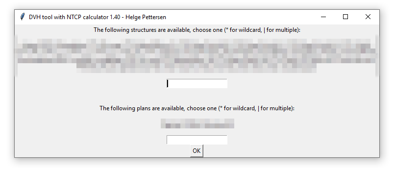
• ECLIPSE files: Most of the options here are similar, but in addition the program supports different organ structures. The file is read out, and all found structures are listed in a dialog when choosing the Load patient folder button. Write a string that matches the wanted structures («Brain*» matches «Brain», «Whole Brain», «Brain L» etc.): Use a wildcard * to match several structures, and a pipe | to include several structures.

The patient toxicity can either be given as another CVS file (to be called «cohort_tox.csv» in the folder above the cohort folder): This file should contain each patient by their filename and toxicity grade. If the patient contained in 1234.csv has grade 3, write a line «1234,3» in the file. Then, choose the wanted toxicity threshold in the program. (2 -> all patients with grade ≥2 are defined as having complications). It is also possible to load the toxicity from the filenames, so that any file with «tox» in the filename is defined as having toxicity. In that case, use toxicity limit 1.

After these settings have been configured, load one or more patient cohorts using the Load patient folder button. This will open a file dialog, where you choose the folder containing the CSV files. The cohort name will be the name of the folder. All the added cohorts will be pooled to a single dataset. The validity of the loaded data may be controlled with the Show DVHs button: patients with tox are shown in red.

The loaded patient sets can be displayed with a range of options and groupings (per plan, per structure) etc. The show DVHs button displays the following menu:

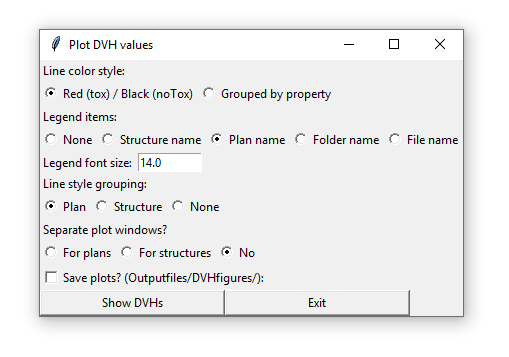
The Show Aggregated DVH Plot button opens a window where all patients within a certain group (structure, plan) can be added together, showing the median / mean DVH for the given plan / structure.

In addition, certain % Dose or % Volume values can be calculated for each patient and stored in output CSV files for further use with the Save DVH values button.

If the LKB model is to be used for calculations, a set of look-up-tables for the gEUD values must be calculated after loading the patient cohorts. This is only performed once per patient (per structure), and is done by clicking the Calculate gEUD splines button. The look-up-tables are stored as cubic splines in the cohort folder (subfolder gEUD), ensuring high interpolation accuracy for all values of n.

The Show gEUD/n button can subsequently be used to display the different gEUD values as functions of n.

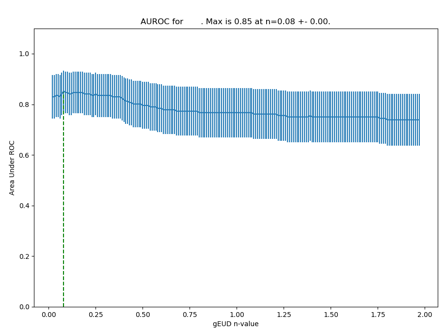
AUROC

In order to identify the strength of different n values for the dataset, it is possible to calculate the AUROC: For each n value, check how many patients are correctly modelled with toxicity using a dose threshold based on their gEUD values (gEUD < threshold -> no tox; gEUD > threshold -> tox). The AUROC for this sensitivity and specificity for this n value calculated, and the n values are varied according to the limits chosen [2].

Choice of NTCP Model

Two methods for calculating the NTCP are supported:

• The logit model , where D is calculated as the dose at a given volume fraction. In that case, choose the % value below, e.g. D20% or D1%. For each patient, this value is calculated from the DVH files.
• The Lyman-Kutcher-Burman (LKB) model [3], [4], in which a the DVH is aggregated to a gEUD value as calculated from a (here created) differential DVH. The n value describes whether the organ is serial or parallel. Then, the two parameters m (population variance) and TD50 (dose giving a 50% probability of toxicity) are used in a cumulative density function (CDF)

In this program, the CDF is substituted by a homotopy perturbation method to increase the computational efficiency [5]:

&space;\right]^{-1},&space;\qquad&space;t=\frac{\mathrm{gEUD}-\mathrm{TD50}}{m\cdot&space;\mathrm{TD50}})

Finding the model parameters of the NTCP model

The main part of the program is to find the model parameters of the chosen NTCP model: a,b for the Logit model, and n,m,TD50 for the LKB model. The bounds of the parameters are defined (or the default values can be kept). Two methods are supplied for the optimization procedure:

• Matrix Minimization: A grid of a given size (matrix size option) is made in 2 (logit) or 3 (LKB) dimensions. For each cell, the error between the calculated NTCP model and the truth (toxicity) is summed over all patient, and the parameters corresponding to the cell containing the lowest error are stored. This is time demanding, especially for the LKB model with large matrix sizes (high granularity of the output parameters).
• Gradient Descent Optimization: Here, an algorithm applying the truncated Newton algorithm [6] for unconstrained optimization of the parameters, together with a basin jumping procedure for locating the global minimum from any identified local minima [7]. The methods are implemented using the scipy.optimize.basinhopping routine [8]. It is substantially quicker compared to the matrix minimization, and can also locate minima with a higher accuracy. This method is configured with a certain number of «basin hoppings», or perturbations from a located minimum. The «temperature» is the expected change in error between minima and the «jump lengths» define the limits of a random variable defining the perturbation for a given parameter.

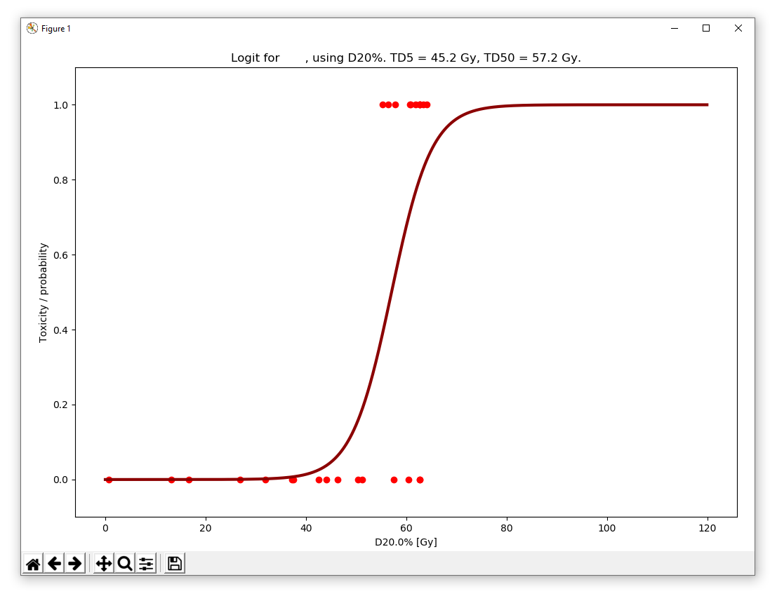
With each optimization method, the error calculation can be as least squares or a Maximum Log Likelihood

,

the latter being more adopted [3]. The chosen method is applied by using the Calculate NTCP button, in which a plot as shown below is displayed (here with D1% and logit):

Calculating the confidence limits of the models

In this part of the program, several approaches have been attempted and compared. In [3], three methods are described:

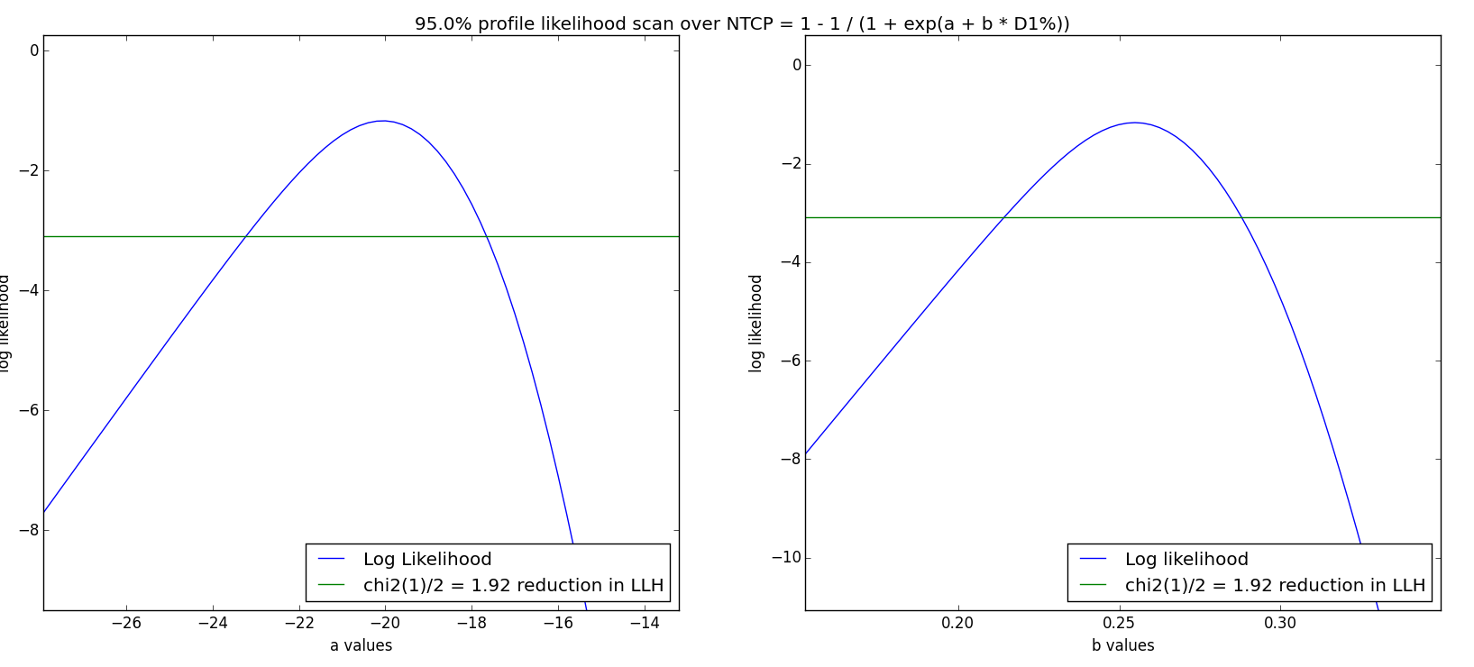
• Profile likelihood: For each parameter, a 1D scan is performed. The Log Likelihood value is drawn as a function of the parameter, with its maximum at the fitted value. Then, the two locations where are identified, where is the critical value with 1 DoF. A 95% confidence interval corresponds to
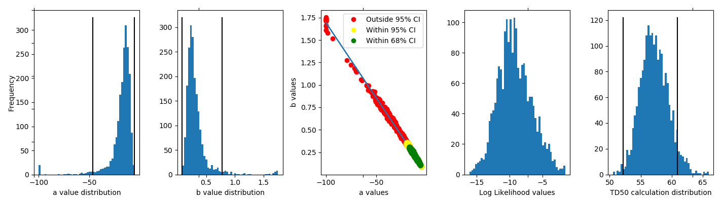
• Non-parametric Bootstrap: This statistical method originates from [9], and is a Monte Carlo-type method to increase the statistical power of a sample. With n patients in the cohort, n patients are chosen at random (with replacement). For each synthetic cohort, a parameter optimization is performed to obtain a new set of parameters a,b or n,m,TD50. The resulting distribution of parameters is used to calculate the statistics such as 95% confidence interval, median parameters etc. This process is repeated 1000-2000 times (chosen as the Number of CI bootstrapping iterations). If the «Use CI median as parameters» is chosen, the median value of this new distribution substitutes the former found optimal parameter set in future NTCP plots (calculate NTCP model after Calculate Confidence Intervals)
• Parametric bootstrap: Similar to the non-parametric bootstrap. Instead of choosing a synthetic cohort, now the cohort it kept but for each patient a random number is generated. If the NTCP calculated from the model fitted paramateters is lower than this value, no complication is assumed, and if complication is assumed. Then, a parameter set is found from this new toxicity cohort: to be repeated 1000-2000 times.

The black lines are bias corrected confidence, intervals, while the green ones are uncorrected.

Using the bootstrap methods, a «pivot» interval can be used as improved CI [10, p. 11], and it is calculated as , Where are the upper and lower limits, respectively, and is the best estimate value from the original distribution.

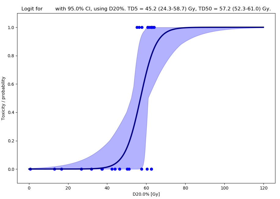
After calculation of the confidence intervals, the Calculate NTCP Model button will display the confidence limits. If the “display each BS model within NTCP CI” option is used, all the individual models (that are within the LLH CI) are drawn on top of the shaded NTCP CI. The error band calculated from the span of bootstrapped models within the confidence interval of the distribution of the variable of interest (TD50).

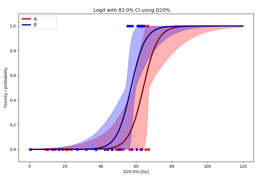
Comparing cohorts

It is possible to compare the NTCP output of two or more cohorts. This is done by adding the wanted data to the left pane, and performing the bootstrap analysis; and then removing / adding a new data set and repeating the analysis. Now, the bootstrap window shows an additional plot (don't close the first NTCP model window!) with the differential TD50 distribution (for logit), and the NTCP/w error display shows both distributions:

Bibliography

• [1] W. McKinney, “Data Structures for Statistical Computing in Python,” in Proceedings of the 9th Python in Science Conference, 2010, pp. 51–56.
• [2] T. Boulé, M. I. G. Fuentes, J. V. Roselló, R. A. Lara, J. L. Torrecilla, and A. L. Plaza, “Clinical comparative study of dose–volume and equivalent uniform dose based predictions in post radiotherapy acute complications,” Acta Oncol., vol. 48, no. 7, pp. 1044–1053, Jan. 2009.
• [3] M. Carolan, B. Oborn, K. Foo, A. Haworth, S. Gulliford, and M. Ebert, “An MLE method for finding LKB NTCP model parameters using Monte Carlo uncertainty estimates,” J. Phys. Conf. Ser., vol. 489, p. 012087, Mar. 2014.
• [4] S. L. Gulliford, M. Partridge, M. R. Sydes, S. Webb, P. M. Evans, and D. P. Dearnaley, “Parameters for the Lyman Kutcher Burman (LKB) model of Normal Tissue Complication Probability (NTCP) for specific rectal complications observed in clinical practise,” Radiother. Oncol., vol. 102, no. 3, pp. 347–351, Mar. 2012.
• [5] Hector Vazquez-Leal, Roberto Castaneda-Sheissa, Uriel Filobello-Nino, Arturo Sarmiento-Reyes, and Jesus Sanchez Orea, “High Accurate Simple Approximation of Normal Distribution Integral,” Math. Probl. Eng., vol. 124029, 2012.
• [6] L. Grippo, F. Lampariello, and S. I. L. Lucid, “A truncated Newton method with nonmonotone line search for unconstrained optimization,” J. Optim. Theory Appl., pp. 401–419, 1989.
• [7] D. J. Wales and J. P. K. Doye, “Global Optimization by Basin-Hopping and the Lowest Energy Structures of Lennard-Jones Clusters Containing up to 110 Atoms,” J. Phys. Chem. A, vol. 101, no. 28, pp. 5111–5116, Jul. 1997.
• [8] E. Jones, E. Oliphant, P. Petersen, and and others, SciPy: Open Source Scientific Tools for Python. 2001.
• [9] B. Efron, “Bootstrap Methods: Another Look at the Jackknife,” Ann. Stat., vol. 7, no. 1, pp. 1–26, 1979.
• [10] D. Banks, “STAT110 lecture: Bootstrap Confidence Intervals.” http://www2.stat.duke.edu/~banks/111-lectures.dir/lect13.pdf