robust_fourier
You want to compute the Fourier transform of a signal, but your signal can be corrupted by outliers? If so, this package is for you even though you will have to say goodbye to the "fast" in Fast Fourier Transform 🏃🙅♀️
🎁 Installation
🐍☁️ PyPI
The package can be installed from PyPI with
pip install robust_fourierIf speed matters for you, you can also install the package with the optional dependency
numba
pip install robust_fourier[fast]🐙📦 GitHub
To install the package from GitHub, you can simply clone the repository
git clone https://github.com/MothNik/robust_fourier.gitFor the following commands, a Makefile is provided to simplify the process. Its use is
optional, but recommended.
From within the repositories root directory, the package can be installed for normal use
# ⚠️ first, activate your virtual environment, e.g., source venv/bin/activate

make install
# equivalent to
pip install --upgrade .
or for development (with all the development dependencies)
# ⚠️ first, activate your virtual environment, e.g., source venv/bin/activate

make install-dev
# equivalent to
pip install --upgrade .["dev"]
⚙️ Setup and 🪛 Development
When working in developer mode, an environment variable has to be added to run certain scripts.
ROBFT_DEVELOPER = true🔎 Code quality
The following checks for black, isort, pyright, mypy, pycodestyle, and
ruff - that are also part of the CI pipeline - can be run with
make black-check
make isort-check
make pyright-check
make mypy-check
make pycodestyle-check
make ruff-check

# or for all at once
make check

# equivalent to
black --check --diff --color ./auxiliary_scripts ./examples ./src ./tests
isort --check --diff --color ./auxiliary_scripts ./examples ./src ./tests
pyright ./auxiliary_scripts ./examples ./src ./tests
mypy ./auxiliary_scripts ./examples ./src ./tests
ruff check ./auxiliary_scripts ./examples ./src ./tests
pycodestyle ./auxiliary_scripts ./examples ./src ./tests --max-line-length=88 --ignore=E203,W503,E704
✅❌ Tests
To run the tests - almost like in the CI pipeline - you can use
make test-xmlcov  # for an XML report
make test-htmlcov  # for an HTML report

# equivalent to
pytest --cov=robust_fourier ./tests -n="auto" --cov-report=xml -x --no-jit
pytest --cov=robust_fourier ./tests -n="auto" --cov-report=html -x --no-jit
for parallelized testing whose coverage report will be stored in the file
./coverage.xml or in the folder ./htmlcov, respectively.
〰️ Hermite functions
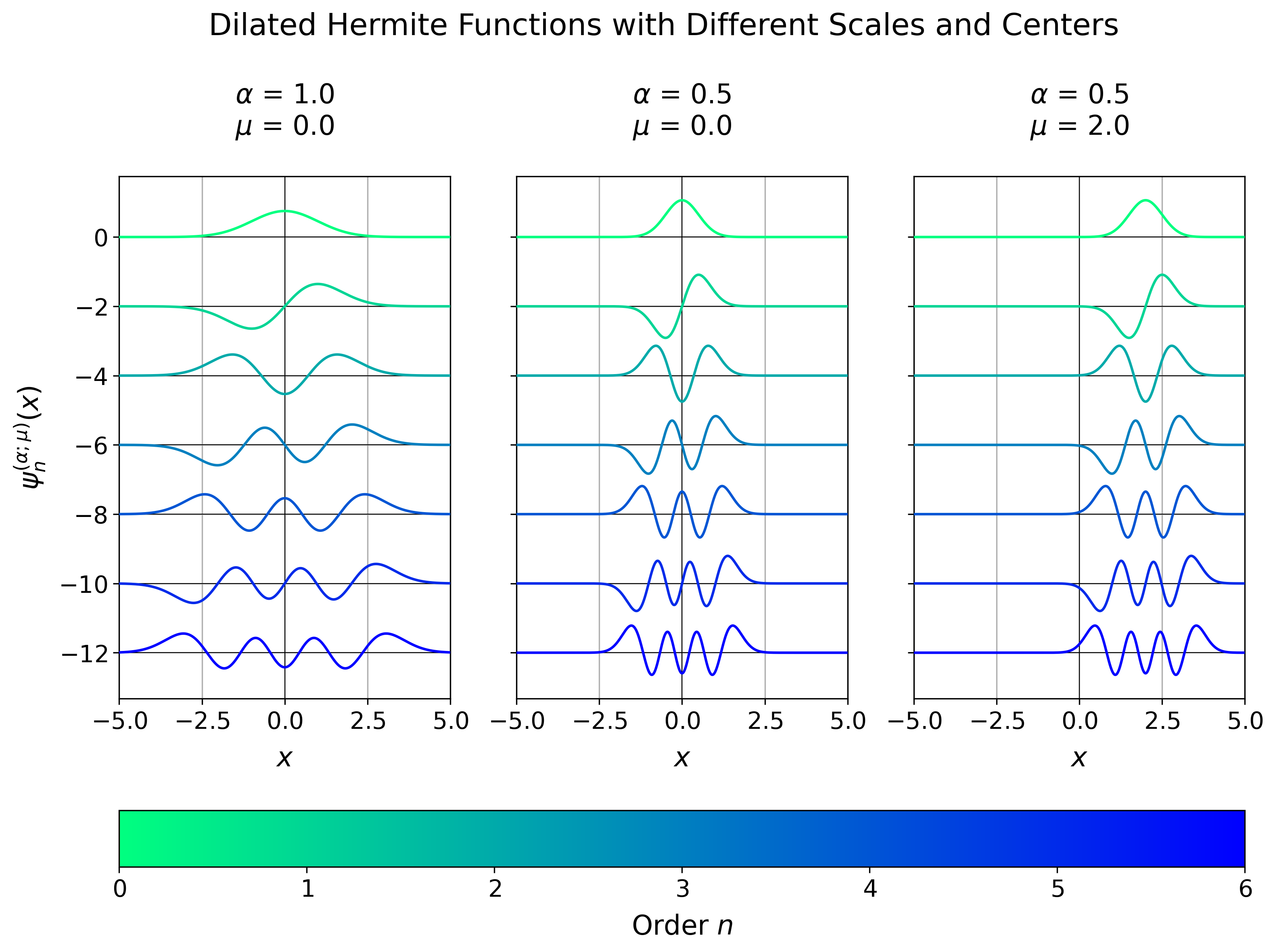
Being the eigenfunctions of the Fourier transform, Hermite functions are excellent candidates for the basis functions for a Least Squares Regression approach to the Fourier transform. However, their evaluation can be a bit tricky.
The module hermite_functions offers a numerically stable way to evaluate Hermite
functions or arbitrary order $n$ and argument - that can be scaled with a factor
$\alpha$ and shifted by a constant $\mu$:

After a slight modification of the definitions in [1], the Hermite functions can be written as
with the Hermite polynomials
With robust_fourier, the Hermite functions can be evaluated for arbitrary orders
using the function interface hermite_function_vander
import numpy as np
from robust_fourier import hermite_function_vander

ORDER_MAX = 25  # the maximum order of the Hermite functions
ALPHA = 2.0  # the scaling factor for the x-variable
MU = -2.0  # the shift of the x-variable

X_FROM = -20.0
X_TO = 20.0
NUM_X = 10_001

x_values = np.linspace(start=X_FROM + MU, stop=X_TO + MU, num=NUM_X)
hermite_vander = hermite_function_vander(
    x=x_values,
    n=ORDER_MAX,
    alpha=ALPHA,
    x_center=MU,
    jit=True,  # will only take effect if Numba is installed
)
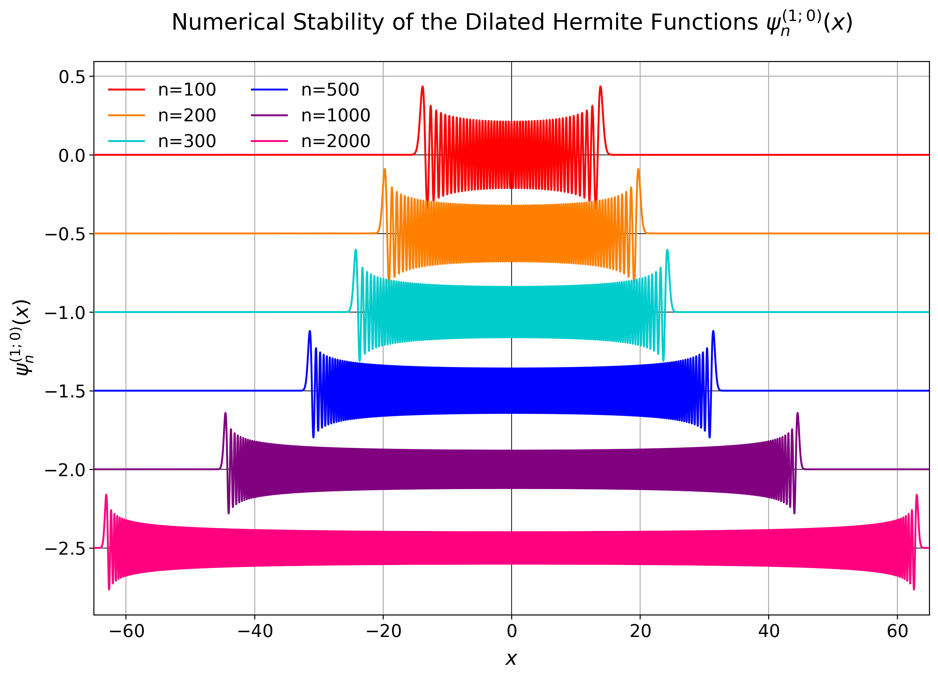
By making use of logarithm tricks, the evaluation that might involve infinitely high polynomial values and at the same time infinitely small Gaussians - that are on top of that scaled by an infinitely high factorial - can be computed safely and yield accurate results.
For doing so, the relation between the dilated and the non-dilated Hermite functions
and the recurrence relation for the Hermite functions
are used, but not directly. Instead, the latest evaluated Hermite function is kept at a value of either -1, 0, or +1 during the recursion and the logarithm of a correction factor is tracked and applied when the respective Hermite function is finally evaluated and stored. This approach is based on [2].
The implementation is tested against a symbolic evaluation with sympy that uses 200
digits of precision and it can be shown that even orders as high as 2,000 can still be
computed even though neither the polynomial, the Gaussian nor the factorial can be
evaluated for this anymore. The factorial for example would already have overflown for
orders of 170 in float64-precision.

As a sanity check, their orthogonality is part of the tests together with a test for the fact that the absolute values of the Hermite functions for real input cannot exceed the value $\frac{1}{\sqrt[4]{\pi\cdot\alpha^{2}}}$.
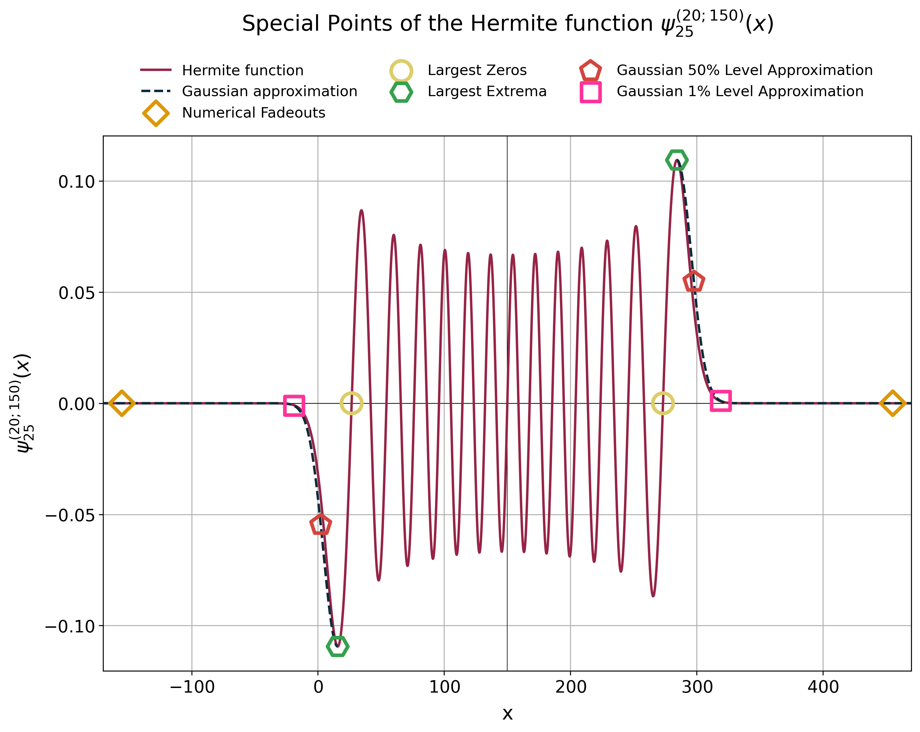
On top of that robust_fourier comes with utility functions to approximate some
special points of the Hermite functions, namely the x-positions of their
- largest root (= outermost zero),
- largest extrema in the outermost oscillation,
- the point where they numerically fade to zero, and
- an approximation of the outermost oscillation (tail) by a conservative Gaussian peak.
import numpy as np
from robust_fourier import hermite_approx

ORDER = 25  # the order of the Hermite functions
ALPHA = 20.0  # the scaling factor for the x-variable
MU = 150.0  # the shift of the x-variable

X_FROM = -65.0
X_TO = 65.0
NUM_X = 100_001

# 1) the x-positions at which the outermost oscillation fades below machine
# precision
x_fadeout = hermite_approx.x_fadeout(
    n=ORDER,
    alpha=ALPHA,
    x_center=MU,
)
# 2) the x-positions of the largest zeros
x_largest_zero = hermite_approx.x_largest_zeros(
    n=ORDER,
    alpha=ALPHA,
    x_center=MU,
)
# 3) the x-positions of the largest extrema
x_largest_extremum = hermite_approx.x_largest_extrema(
    n=ORDER,
    alpha=ALPHA,
    x_center=MU,
)

# 4) the Gaussian approximation of the outermost oscillation ...
left_gaussian, right_gaussian = hermite_approx.get_tail_gauss_fit(
    n=ORDER,
    alpha=ALPHA,
    x_center=MU,
)
# ... which is solved for the 50% level
x_left_fifty_percent = left_gaussian.solve_for_y_fraction(y_fraction=0.5)
x_right_fifty_percent = right_gaussian.solve_for_y_fraction(y_fraction=0.5)
# ... but can also be evaluated for all x-values
x_values = np.linspace(start=X_FROM + MU, stop=X_TO + MU, num=NUM_X)
left_gaussian_values = left_gaussian(x=x_values)
right_gaussian_values = right_gaussian(x=x_values)

# 5) the Gaussian approximation is also solved for the 1% interval as a more
# realistic (less conservative) approximation of the fadeout point
x_one_percent = hermite_approx.x_tail_drop_to_fraction(
    n=ORDER,
    y_fraction=0.01,
    alpha=ALPHA,
    x_center=MU,
).ravel()

🧮 Chebyshev Polynomials
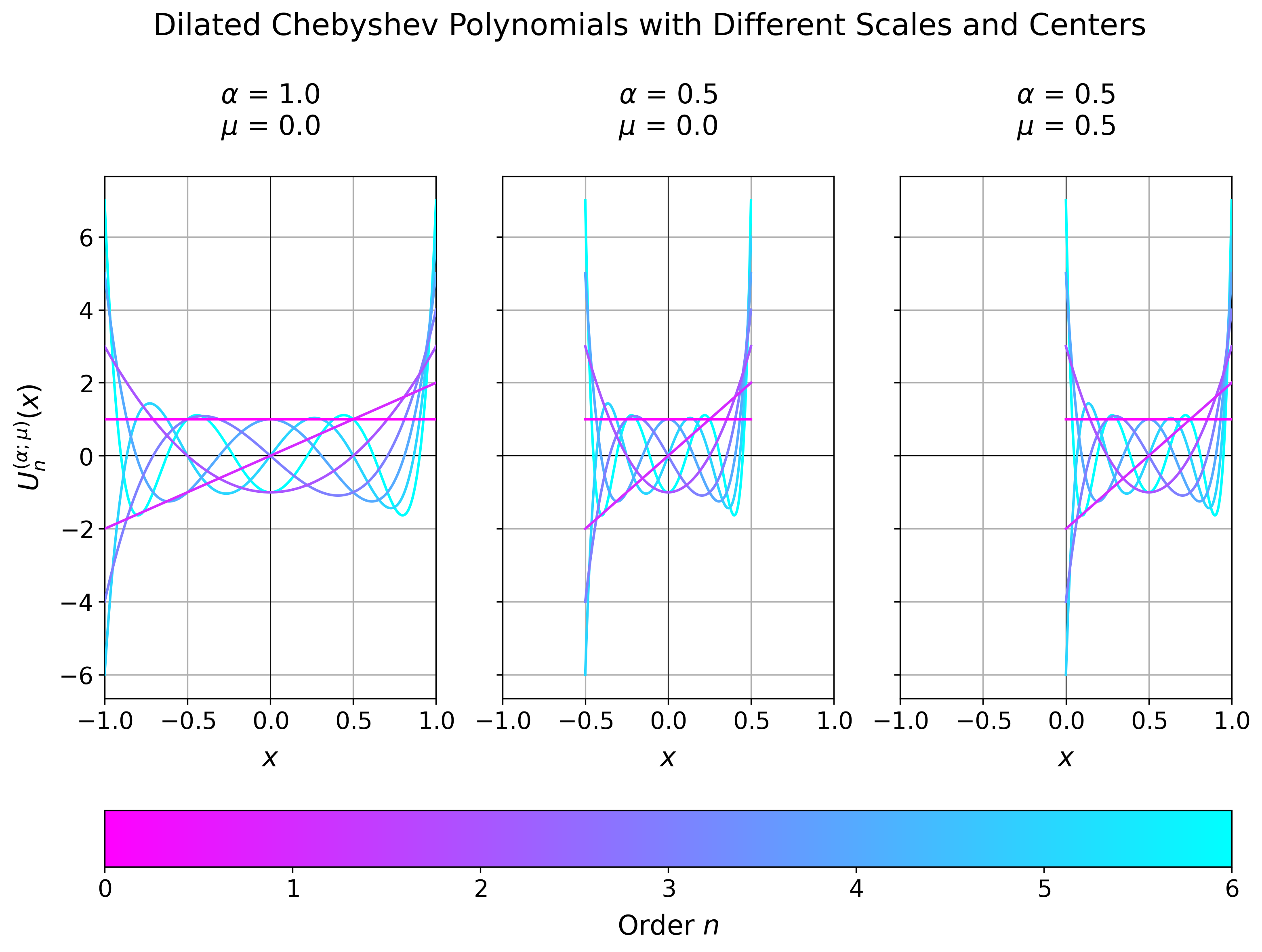
Even though the Hermite functions have some nice properties, they are not necessarily the best choice for the Fourier transform. Choosing their scaling parameter $\alpha$ can be a bit tricky. Therefore [3] suggests using Chebyshev polynomials instead. They are only defined on the interval $[-1, 1]$ and can be scaled and shifted to fit the interval $[\mu - \alpha, \mu + \alpha]$ like
for the first kind and
for the second kind. In [[3]](#references) the second kind $U$ is used, but the first
kind $T$ is also implemented in `robust_fourier`
```python
import numpy as np
from robust_fourier import chebyshev_polyvander
ORDER_MAX = 10 # the maximum order of the Chebyshev polynomials
ALPHA = 0.5 # the scaling factor for the x-variable
MU = 0.5 # the shift of the x-variable
X_FROM = -0.5
X_TO = 0.5
NUM_X = 10_001
x_values = np.linspace(start=X_FROM + MU, stop=X_TO + MU, num=NUM_X)
chebyshev_vander_first_kind = chebyshev_polyvander(
x=x_values,
n=ORDER_MAX,
alpha=ALPHA,
x_center=MU,
kind="first",
jit=True, # will only take effect if Numba is installed
)
chebyshev_vander_second_kind = chebyshev_polyvander(
x=x_values,
n=ORDER_MAX,
alpha=ALPHA,
x_center=MU,
kind="second",
jit=True, # will only take effect if Numba is installed
)
# alternatively, both kinds can be computed in one go because this is how they are
# computed internally to achieve maximum accuracy
(
chebyshev_vander_first_kind,
chebyshev_vander_second_kind,
) = chebyshev_polyvander(
x=x_values,
n=ORDER_MAX,
alpha=ALPHA,
x_center=MU,
kind="both",
jit=True, # will only take effect if Numba is installed
)
```


