Project aimed at stores' sales prediction

The project uses the dataset from Kaggle platform.uj

Dataset description

The dataset contains the information about the daily sales of Favorita stores located in Ecuador per day from January 2013 to August 2017. The whole data consists of several .csv files.

– The train.csv file gives the info about the sales of a certain family of products('family') in a certain store('store_nbr') on a certain day('date') where the target variable 'sales' stands for the number of item (or number of kilos since some items are sold in fractional units, e.g. 2.5 kilos of cheese) of this family sold on this day. Variable 'onpromotion' gives the total number of items in a product family that were being promoted at a store at a given date. This file contains the info from 1st January, 2013 to 15th August, 2017.

– The test.csv file has the same info as train.csv except for the target variable 'sales'. The main challenge is to predict this variable on there days. This file contains the info from 16th to 31st August, 2017.

– The oil.csv file contains the information about the oil prices for the given period.

– The holiday_events.csv file represents the info about different holidays and events in Ecuador for the given period with its characterictics(type, status, location, name, was it transferred to another day or not).

– The stores.csv file contains the info about the stores(number, city, state, type, cluster).

– The sample_submission.csv file is the example of the file needed to be loaded to Kaggle for getting the results.

– The transactions.csv file gives the info about the number of transactions done in a certain store on a given day. However, there's no such info for the test part of the dataset, so we won't use this file.

The goal of the problem

The goal is to build a model for making a prediction of the target variable 'sales' for 16 days from 16th to 31st August, 2017. That actually means that we need to make a separate prediction of the variable 'sales' for every item family in every store for every day during the given period.

Multiple time series technique

Splitting the data by many distinct time series for every unique combination store-item and making an individual prediction for each of them was empirically found to be much better than a staightforward prediction without such splitting.

Validation methods

The TimeSeriesSplit() from Sklearn with n_splits=N_SPLITS (the default value N_SPLITS = 5 is set in src/store_sales/modules/constants.py file) was chosen for performing the cross-validation technique. It means that there will be 5 distinct splits for each time series with the fixed size of the test part equal to 278 days. Its implementation includes the method called Expanding Window and well balanced in terms of computational cost and robustness. Standard Time Series Split, Sliding Window and Nested Cross Validation were among alternatives.

Metrics

– Since the sales of some items are close to zero or exactly zero, there was no point in using a default MAPE metric for getting a percentage error.

– That's why WMAPE (Weighted Mean Absolute Percentage Error) was chosen as the main one since it's much less sensitive to zero values of the target variable.

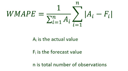
– The final value of the metric is calculated as mean MAE (Mean Absolute Error) across all splits in all distict time series divided by the mean value of the target variable.

Modeling

– We decided to use models based on the gradient boosting principle. It a nutshell, it means that we have multiple consistent models making a prediction based on the previous models' mistakes so that the metric's value is optimized per iteration – One of the models we used is the XBGRegressor from XGBoost. – For this model we used Optuna library for hyperparameter optimization. We set a range of values for each hyperparameter and found optimal ones with help of Optuna tools. The function that finds optimal hyperparameters for XGBRegressor within set boundaries is optimize_xgboost_params_with_optuna() in functions.py. – We decided to choose a random subset of 5 different shops for this task since it would have taken too much time otherwise.

Development

1. Clone this repository to your machine (probably using your IDE, I use VS Code).
2. Download the dataset. Create a folder path data/raw_data in the root directory of the project and save all .csv files there. The constant DATA_PATH in src/store_sales/constants.py is resposible for this path.
3. Make sure Python 3.12.3 and Poetry are installed on your machine (I use Poetry 1.8.2).
4. Install all Poetry dependencies via your terminal:

poetry install 

After that make sure that the virual environment is indeed activated:

poetry env list

If the virtual environment is activated, there will be something like ".venv (Activated)" in the output. If it's not (the list is empty), then you should activate it manually. Run in your teminal:

poetry shell

And make sure that after this command the virtual env is activated. The .venv folder in the root of the project is likely to appear and the following command will tell you that Python from .venv/bin/python is used.

which python

5. Run the split_and_prepare_data.py script for splitting the data and preparing it for the EDA separately so that it's guaranteed there won't be data leakage from future to past. There's a click command line interface implemented so that you can set the paths to input and output folders manually. Navigate to the folder with scripts (as for us, they are in src/store_sales/scripts folder in the root directory of the project). Then run in your terminal:

python split_and_prepare_data.py --raw_data_folder_path <path to the folder with raw data> --prepared_for_eda_data_folder_path <path to the output folder> 

Or you can also run this script as a Poetry script, i.e. from any current path, without the need for navigating to the folder with scripts. For doing this just run in your terminal:

split_and_prepare_data --raw_data_folder_path <path to the folder with raw data> --prepared_for_eda_data_folder_path <path to the output folder>

The default values of these paths are set in src/store_sales/modules/constants.py file (RAW_DATA_FOLDER_PATH and PREPARED_FOR_EDA_DATA_FOLDER_PATH respectively).

Streamlit dashboard (optional)

After the data is split into train and test parts and prepared, it's time to perform the Exploratory Data Analysis on the train part. While doing that, we created some plots for finding out some possible implicit dependencies in the data for constructing a better prediction model. We decided to create an interactive dashboard using the Streamlit tools for a more convenient way to explore the data where you can decide which plot and its categories to view. Navigate to the folder with scripts and then run in your terminal:

streamlit run streamlit_app.py 

Then there will be your Local URL displayed (probably http://localhost:8501). Copy it and paste to your browser and enjoy using the interactive dashboard. The path to the file used for creating the dashboard is set in src/store_sales/modules/constants.py file (DATA_FOR_STREAMLIT_PATH variable).

6. Then you should run the add_new_features.py script for adding certain new features (which might be useful according to the Exploratory Data Analysis). There's also a click command line interface. Same, at first navigate to the folder with scripts. Then run in your terminal:

python add_new_features.py --input_data_folder_path <path to the folder with input data> --prepared_final_data_folder_path <path to the output folder> 

Or you can also run this script as a Poetry script, i.e. from any current path, without the need for navigating to the folder with scripts. For doing this just run in your terminal:

add_new_features --input_data_folder_path <path to the folder with input data> --prepared_final_data_folder_path <path to the output folder> 

The default values of these paths are also set in src/store_sales/modules/constants.py file (PREPARED_FOR_EDA_DATA_FOLDER_PATH and PREPARED_FINAL_DATA_FOLDER_PATH respectively). Pay attention to the fact that the value of the --input_data_folder_path parameter MUST BE THE SAME as the value of the --prepared_final_data_folder_path parameter from the 5th section since data preparation and adding new features are performed sequentially. That's why the default value of these variables are same and refer to a single constant from constants.py.

7. After choosing the model and optimizing its hyperparameters (you can read about it in the Modeling section above) we decided to save both cross-validation metrics and fitted models that can be used for future predicts in the format that would be convenient for storing and reusing in the future distinctly for each pair (store, item_family). The tool that fits this task perfectly is MLFlow that lets you efficiently perform management of your models and experiments together with its artifacts and metadata (metrics, parameters, tags, etc). You can read more about MLFlow via link above.

We also decided to save metrics and models locally using a .json file for metrics and a .pkl file for models. Pay attention to the fact that .pkl files aren't human-readable since they are binary.

For saving your metrics and models your should run the save_and_log_data.py script. The script will find optimal hyperparameters within boundaries set in optimize_xgboost_params_with_optuna() in src/store_sales/hyperparameters_optimization.py, use the optimized model for getting cross-validation models and metrics, save them locally and, if you want, log them to the MLFlow server. The default URI of the server is set as "http://127.0.0.1:8080" in src/store_sales/modules/constants.py file as well as the default name of the experiment. For runnig the script navigate to the folder with script files as it was described in sections 5-6. Then run in your terminal:

python save_and_log_data.py --metrics_folder_path <path to the folder where you want to save metrics> --models_folder_path <path to the folder where you want to save models> --send_to_server <True if you want to log your models and metrics to the MLFlow server and False otherwise, the default value is True>

Or you can also run this script as a Poetry script, i.e. from any current path, without the need for navigating to the folder with scripts. For doing this just run in your terminal:

save_and_log_data --metrics_folder_path <path to the folder where you want to save metrics> --models_folder_path <path to the folder where you want to save models> --send_to_server <True if you want to log your models and metrics to the MLFlow server and False otherwise, the default value is True>

The default values of these paths are set in src/store_sales/modules/constants.py file (METRICS_FOLDER_PATH and MODELS_FOLDER_PATH respectively).

8. Some libraries (Ruff, Black) for effective code usage and formatting were also used. For using them run in your terminal:

ruff check <path to the folder with your .py files>

black <path to the folder with your .py files>